This is chapter 2 in my forthcoming book Can we avoid another financial crisis? (Polity Press, April 2017)

Microeconomics, Macroeconomics and Complexity

Since 1976, Robert Lucas—he of the confidence that the “problem of depression prevention has been solved”—has dominated the development of mainstream macroeconomics with the proposition that good macroeconomic theory could only be developed from microeconomic foundations. Arguing that “the structure of an econometric model consists of optimal decision rules of economic agents” (Lucas, 1976, p. 13), Lucas insisted that to be valid, a macroeconomic model had to be derived from the microeconomic theory of the behaviour of utility-maximizing consumers and profit-maximizing firms.

In fact, Lucas’s methodological precept—that macro level phenomena can and in fact must be derived from micro-level foundations—had been invalidated before he stated it. As long ago as 1953 (Gorman, 1953), mathematical economists posed the question of whether what microeconomic theory predicted about the behaviour of an isolated consumer applied at the level of the market. They concluded, reluctantly, that it did not:

market demand functions need not satisfy in any way the classical restrictions which characterize consumer demand functions… The importance of the above results is clear: strong restrictions are needed in order to justify the hypothesis that a market demand function has the characteristics of a consumer demand function. Only in special cases can an economy be expected to act as an ‘idealized consumer’. The utility hypothesis tells us nothing about market demand unless it is augmented by additional requirements.’ (Shafer and Sonnenschein, 1993, p. 671-72)

What they showed was that if you took two or more consumers with different tastes and different income sources, consuming two or more goods whose relative consumption levels changed as incomes rose (because some goods are luxuries and others are necessities), then the resulting market demand curves could have almost any shape at all.[1] They didn’t have to slope downwards, as economics textbooks asserted they did.

This doesn’t mean that demand for an actual commodity in an actual economy will fall if its price falls, rather than rise. It means instead that this empirical regularity must be due to features that the model of a single consumer’s behaviour omits. The obvious candidate for the key missing feature is the distribution of income between consumers, which will change when prices change.

The reason that aggregating individual downward sloping demand curve results in a market demand curve that can have any shape at all is simple to understand, but—for those raised in the mainstream tradition—very difficult to accept. The individual demand curve is derived by assuming that relative prices can change without affecting the consumer’s income. This assumption can’t be made when you consider all of society—which you must do when aggregating individual demand to derive a market demand curve—because changing relative prices will change relative incomes as well.

Since changes in relative prices change the distribution of income, and therefore the distribution of demand between different markets, demand for a good may fall when its price falls, because the price fall reduces the income of its customers more than the lower relative price boosts demand (I give a simple illustration of this in Keen, 2011 on pages 51-53).

The sensible reaction to this discovery is that individual demand functions can be grouped only if changing relative prices won’t substantially change income distribution within the group. This is valid if you aggregate all wage earners into a group called “Workers”, all profit earners into a group called “Capitalists”, and all rent earners into a group called “Bankers”—or in other words, if you start your analysis from the level of social classes. Alan Kirman proposed such a response almost 3 decades ago:

If we are to progress further we may well be forced to theories in terms of groups who have collectively coherent behavior. Thus demand and expenditure functions if they are to be set against reality must be defined at some reasonably high level of aggregation. The idea that we should start at the level of the isolated individual is one which we may well have to abandon. (Kirman, 1989, p. 138)

Unfortunately, the reaction of the mainstream was less enlightened: rather than accepting this discovery, they looked for conditions under which it could be ignored. These conditions are absurd—they amount to assuming that all individuals and all commodities are identical. But the desire to maintain the mainstream methodology of constructing macro-level models by simply extrapolating from individual level models won out over realism.

The first economist to derive this result, William Gorman, argued that it was “intuitively reasonable” to make what is in fact an absurd assumption that changing the distribution of income does not alter consumption:

The necessary and sufficient condition quoted above is intuitively reasonable. It says, in effect, that an extra unit of purchasing power should be spent in the same way no matter to whom it is given. (Gorman, 1953, pp. 63-64. Emphasis added)

Paul Samuelson, who arguably did more to create Neoclassical economics than any other 20^th century economist, conceded that unrelated individual demand curves could not be aggregated to yield market demand curves that behaved like individual ones. But he then asserted that a “family ordinal social welfare function” could be derived “since blood is thicker than water”: family members could be assumed to redistribute income between each other “so as to keep the ‘marginal social significance of every dollar’ equal” (Samuelson, 1956, pp. 10-11. Emphasis added). He then blithely extended this vision of a happy family to the whole of society:

“The same argument will apply to all of society if optimal reallocations of income can be assumed to keep the ethical worth of each person’s marginal dollar equal” (Samuelson, 1956, p. 21. Emphasis added).

The textbooks from which mainstream economists learn their craft shielded students from the absurdity of these responses, and thus set them up to unconsciously make inane rationalisations themselves when they later constructed what they believed were microeconomically sound models of macroeconomics, based on the fiction of “a representative consumer”. Hal Varian’s advanced mainstream text Microeconomic Analysis (first published in 1978) reassured Masters and PhD students that this procedure was valid:

“it is sometimes convenient to think of the aggregate demand as the demand of some ‘representative consumer’… The conditions under which this can be done are rather stringent, but a discussion of this issue is beyond the scope of this book…” (Varian, 1984, p. 268)

and portrayed Gorman’s intuitively ridiculous rationalisation as reasonable:

Suppose that all individual consumers’ indirect utility functions take the Gorman form … [where] … the marginal propensity to consume good j is independent of the level of income of any consumer and also constant across consumers … This demand function can in fact be generated by a representative consumer. (Varian, 1992, pp. 153-154. Emphasis added. Curiously the innocuous word “generated” in this edition replaced the more loaded word “rationalized” in the 1984 edition)

It’s then little wonder that, decades later, macroeconomic models, painstakingly derived from microeconomic foundations—in the false belief that it was legitimate to scale the individual up to the level of society, and thus to ignore the distribution of income—failed to foresee the biggest economic event since the Great Depression.

So macroeconomics cannot be derived from microeconomics. But this does not mean that “The pursuit of a widely accepted analytical macroeconomic core, in which to locate discussions and extensions, may be a pipe dream”, as Blanchard put it. There is a way to derive macroeconomic models by starting from foundations that all economists must agree upon. But to actually do this, economists have to embrace a concept that to date the mainstream has avoided: complexity.

The discovery that higher order phenomena cannot be directly extrapolated from lower order systems is a commonplace conclusion in genuine sciences today: it’s known as the “emergence” issue in complex systems (Nicolis and Prigogine, 1971, Ramos-Martin, 2003). The dominant characteristics of a complex system come from the interactions between its entities, rather than from the properties of a single entity considered in isolation.

My favourite instance of it is the behaviour of water. If one could, and in fact, one had to derive macroscopic behaviour from microscopic principles, then weather forecasters would have to derive the myriad properties of the weather from the characteristics of a single molecule of H₂O. This would entail showing how, under appropriate conditions, a “water molecule” could become an “ice molecule”, a “steam molecule”, or—my personal favourite—a “snowflake molecule”. In fact, the wonderful properties of water occur, not because of the properties of individual H₂O molecules themselves, but because of interactions between lots of (identical) H₂O molecules.

The fallacy in the belief that higher level phenomena (like macroeconomics) had to be, or even could be, derived from lower level phenomena (like microeconomics) was pointed out clearly in 1972—again, before Lucas wrote—by the Physics Nobel Laureate Philip Anderson:

The main fallacy in this kind of thinking is that the reductionist hypothesis does not by any means imply a “constructionist” one: The ability to reduce everything to simple fundamental laws does not imply the ability to start from those laws and reconstruct the universe. (Anderson, 1972, p. 393. Emphasis added)

He specifically rejected the approach of extrapolating from the “micro” to the “macro” within physics. If this rejection applies to the behaviour of fundamental particles, how much more so does it apply to the behaviour of people?:

The behavior of large and complex aggregates of elementary particles, it turns out, is not to be understood in terms of a simple extrapolation of the properties of a few particles. Instead, at each level of complexity entirely new properties appear, and the understanding of the new behaviors requires research which I think is as fundamental in its nature as any other. (Anderson, 1972 , p. 393)

Anderson was willing to entertain that there was a hierarchy to science, so that:

one may array the sciences roughly linearly in a hierarchy, according to the idea: “The elementary entities of science X obey the laws of science Y”

Table 1: Anderson’s hierarchical ranking of sciences (adapted from Anderson 1972, p. 393)

X	Y
Solid state or many-body physics	Elementary particle physics
Chemistry	Many-body physics
Molecular biology	Chemistry
Cell biology	Molecular biology
…	…
Psychology	Physiology
Social sciences	Psychology

But he rejected the idea that any science in the X column could simply be treated as the applied version of the relevant science in the Y column:

But this hierarchy does not imply that science X is “just applied Y”. At each stage entirely new laws, concepts, and generalizations are necessary, requiring inspiration and creativity to just as great a degree as in the previous one. Psychology is not applied biology, nor is biology applied chemistry. (Anderson, 1972 , p. 393)

Nor is macroeconomics applied microeconomics. Mainstream economists have accidentally proven Anderson right by their attempt to reduce macroeconomics to applied microeconomics, firstly by proving it was impossible, and secondly by ignoring this proof, and consequently developing macroeconomic models that blindsided economists to the biggest economic event of the last seventy years.

The impossibility of taking a “constructionist” approach to macroeconomics, as Anderson described it, means that if we are to derive a decent macroeconomics, we have to start at the level of the macroeconomy itself. This is the approach of complex systems theorists: to work from the structure of the system they are analysing, since this structure, properly laid out, will contain the interactions between the system’s entities that give it its dominant characteristics.

This was how the first complex systems models of physical phenomena were derived: the so-called “many body problem” in astrophysics, and the problem of turbulence in fluid flow.

Newton’s equation for gravitational attraction explained how a predictable elliptical orbit results from the gravitational attraction of the Sun and a single planet, but it could not be generalised to explain the dynamics of the multi-planet system in which we actually live. The great French mathematician Henri Poincare discovered in 1899 that the orbits would be what we now call “chaotic”: even with a set of equations to describe their motion, accurate prediction of their future motion would require infinite precision of measurement of their positions and velocities today. As astrophysicist Scott Tremaine put it, since infinite accuracy of measurement is impossible, then “for practical purposes the positions of the planets are unpredictable further than about a hundred million years in the future”:

As an example, shifting your pencil from one side of your desk to the other today could change the gravitational forces on Jupiter enough to shift its position from one side of the Sun to the other a billion years from now. The unpredictability of the solar system over very long times is of course ironic since this was the prototypical system that inspired Laplacian determinism. (Tremaine, 2011)

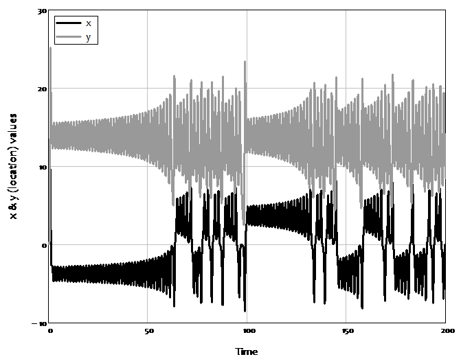
This unpredictable nature of complex systems led to the original description of the field as “Chaos Theory”, because in place of the regular cyclical patterns of harmonic systems there appeared to be no pattern at all in complex ones. A good illustration of this is Figure 1, which plots the superficially chaotic behaviour over time of two of the three variables in the complex systems model of the weather developed by Edward Lorenz in 1963 (Lorenz, 1963).

Figure 1: The apparent chaos in Lorenz’s weather model

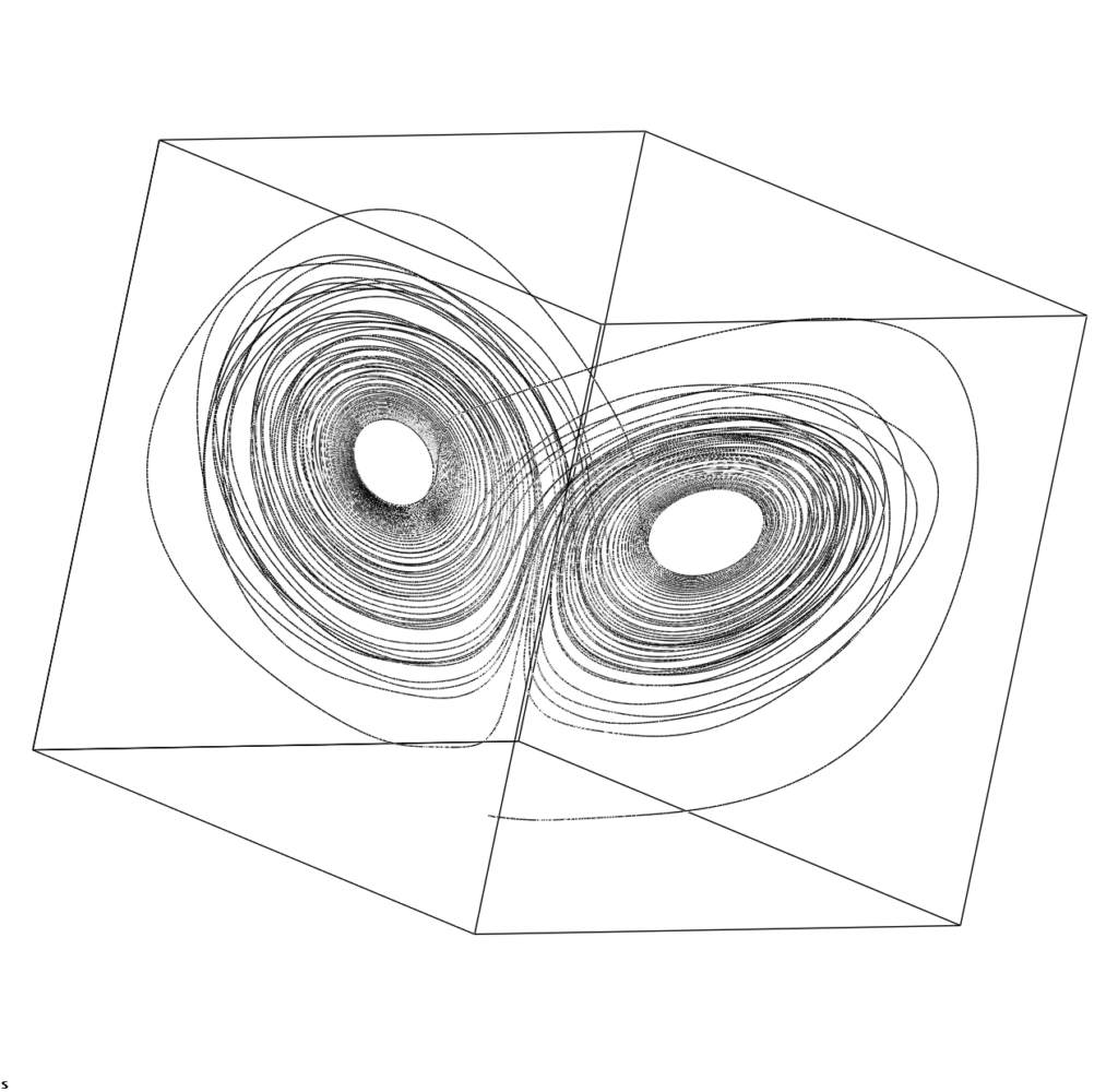
However, long term unpredictability means neither a total lack of predictability, nor a lack of structure. You almost surely know of the phrase “the butterfly effect”: the saying that a butterfly flapping or not flapping its wings in Brazil can make the difference between the occurrence or not of a hurricane in China. The butterfly metaphor was inspired by plotting the three variables in Lorenz’s model against each other in a “3D” diagram. The apparently chaotic behaviour of the x and z variables in the “2D” plot of Figure 2 gives way to the beautiful “wings of a butterfly” pattern shown in Figure 2 when all three dimensions of the model are plotted against each other.

Figure 2: Lorenz’s “Butterfly” weather model—the same data as in Figure 1 in 3 dimensions

The saying does not mean that butterflies cause hurricanes, but rather that imperceptible differences in initial conditions can make it essentially impossible to predict the path of complex systems like the weather after a relatively short period of time. Though this eliminates the capacity to make truly long term weather forecasts, the capacity to forecast for a finite but still significant period of time is the basis of the success of modern meteorology.

Lorenz developed his model because he was dissatisfied with the linear models that were used at the time to make weather forecasts, when meteorologists knew that the key phenomena in weather involved key variables—such as the temperature and density of a gas—interacting with each other in non-additive ways. Meteorologists already had nonlinear equations for fluid flow, but these were too complicated to simulate on computers in Lorenz’s day. So he produced a drastically simplified model of fluid flow with just 3 equations and 3 parameters (constants)—and yet this extremely simple model developed extremely complex cycles which captured the essence of the instability in the weather itself.

Lorenz’s very simple model generated sustained cycles because, for realistic parameter values, its three equilibria were all unstable. Rather than dynamics involving a disturbance followed by a return to equilibrium, as happens with stable linear models, the dynamics involved the system being far from equilibrium at all times. To apply Lorenz’s insight, meteorologists had to abandon their linear, equilibrium models—which they willingly did—and develop nonlinear ones which could be simulated on computers. This has led, over the last half century, to far more accurate weather forecasting than was possible with linear models.

The failure of economics to develop anything like the same capacity is partly because the economy is far less predictable than the weather, given human agency, as Hayekian economists justifiably argue. But it is also due to the insistence of mainstream economists on the false modelling strategies of deriving macroeconomics by extrapolation from microeconomics, and of assuming that the economy is a stable system that always returns to equilibrium after a disturbance.

Abandoning these false modelling procedures does not lead, as Blanchard fears, to an inability to develop macroeconomic models from a “widely accepted analytical macroeconomic core”. Neoclassical macroeconomists have tried to derive macroeconomics from the wrong end—that of the individual rather than the economy—and have done so in a way that glossed over the aggregation problems that entails by pretending that an isolated individual can be scaled up to the aggregate level. It is certainly sounder—and may well be easier—to proceed in the reverse direction, by starting from aggregate statements that are true by definition, and then by disaggregating those when more detail is required. In other words, a “core” exists in the very definitions of macroeconomics.

Using these definitions, it is possible to develop, from first principles that no macroeconomist can dispute, a model that does four things that no DSGE model can do: it generates endogenous cycles; it reproduces the tendency to crisis that Minsky argued was endemic to capitalism; it explains the growth of inequality over the last 50 years; and it implies that the crisis will be preceded, as it indeed was, by a “Great Moderation” in employment and inflation.

The three core definitions from which a rudimentary macro-founded macroeconomic model can be derived are the employment rate (the ratio of those with a job to total population, as an indicator of both the level of economic activity and the bargaining power of workers), the wages share of output (the ratio of wages to GDP, as an indicator of the distribution of income), and, as Minsky insisted, the private debt to GDP ratio.[1]

When put in dynamic form, these definitions lead to not merely “intuitively reasonable” statements, but statements that are true by definition:

• The employment rate (the percentage of the population that has a job) will rise if the rate of economic growth (in percent per year) exceeds the sum of population growth and labour productivity growth;
• The percentage share of wages in GDP will rise if wage demands exceed the growth in labour productivity; and
• The debt to GDP ratio will rise if private debt grows faster than GDP.

These are simply truisms. To turn them into an economic model, we have to postulate some relationships between the key entities in the system: between employment and wages, between profit and investment, and between debt, profits and investment.

Here an insight from complex systems analysis is extremely important: a simple model can explain most of the behaviour of a complex system, because most of its complexity come from the fact that its components interact—and not from the well-specified behaviour of the individual components themselves (Goldenfeld and Kadanoff, 1999). So the simplest possible relationships may still reveal the core properties of the dynamic system—which in this case is the economy itself.

In this instance, the simplest possible relationships are:

• Output is a multiple of the installed capital stock;
• Employment is a multiple of output;
• The rate of change of the wage is a linear function of the employment rate;
• Investment is a linear function of the rate of profit;
• Debt finances investment in excess of profits; and
• Population and labour productivity grow at constant rates.

The resulting model is far less complicated than even a plain vanilla DSGE model: it has just 3 variables, 9 parameters, and no random terms.[2] It omits many obvious features of the real world, from government and bankruptcy provisions at one extreme to Ponzi lending to households by the banking sector at the other. As such, there are many features of the real world that cannot be captured without extending its simple foundations.[3]

However, even at this simple level, its behaviour is far more complex than even the most advanced DSGE model, for at least three reasons. Firstly, the relationships between variables in this model aren’t constrained to be simply additive, as they are in the vast majority of DSGE models: changes in one variable can therefore compound changes in another, leading to changes in trends that a linear DSGE model cannot capture. Secondly, non-equilibrium behaviour isn’t ruled out by assumption, as in DSGE models: the entire range of outcomes that can happen is considered, and not just those that are either compatible with or lead towards equilibrium. Thirdly, the finance sector, which is ignored in DSGE models (or at best treated merely as a source of “frictions” that slow down the convergence to equilibrium), is included in a simple but fundamental way in this model, by the empirically confirmed assumption that investment in excess of profits is debt-financed (Fama and French, 1999a, p. 1954).[4]

The model generates two feasible outcomes, depending on how willing capitalists are to invest. A lower level of willingness leads to equilibrium. A higher level leads to crisis.

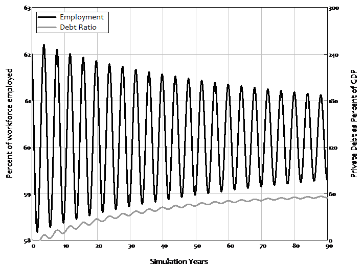
With a low propensity to invest, the system stabilises: the debt ratio rises from zero to a constant level, while cycles in the employment rate and wages share gradually converge on equilibrium values. This process is shown in Figure 3, which plots the employment rate and the debt ratio.

Figure 3: Equilibrium with less optimistic capitalists

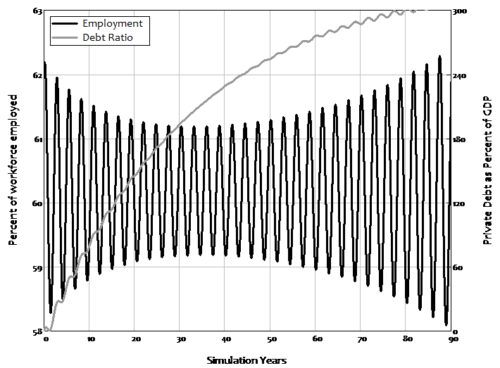
With a higher propensity to invest comes the debt-driven crisis that Minsky predicted, and which we experienced in 2008. However, something that Minsky did not predict, but which did happen in the real world, also occurs in this model: the crisis is preceded by a period of apparent economic tranquillity that superficially looks the same as the transition to equilibrium in the good outcome. Before the crisis begins, there is a period of diminishing volatility in unemployment, as shown in Figure 4: the cycles in employment (and wages share) diminish, and at a faster rate than the convergence to equilibrium in the good outcome shown in Figure 3.

But then the cycles start to rise again: apparent moderation gives way to increased volatility, and ultimately a complete collapse of the model, as the employment rate and wages share of output collapse to zero and the debt to GDP ratio rises to infinity. This model, derived simply from the incontestable foundations of macroeconomic definitions, implies that the “Great Moderation”, far from being a sign of good economic management as mainstream economists interpreted it (Blanchard et al., 2010, p. 3), was actually a warning of an approaching crisis.

Figure 4: Crisis with more optimistic capitalists

The difference between the good and bad outcomes is the factor Minsky insisted was crucial to understanding capitalism, but which is absent from mainstream DSGE models: the level of private debt. It stabilizes at a low level in the good outcome, but reaches a high level and does not stabilize in the bad outcome.

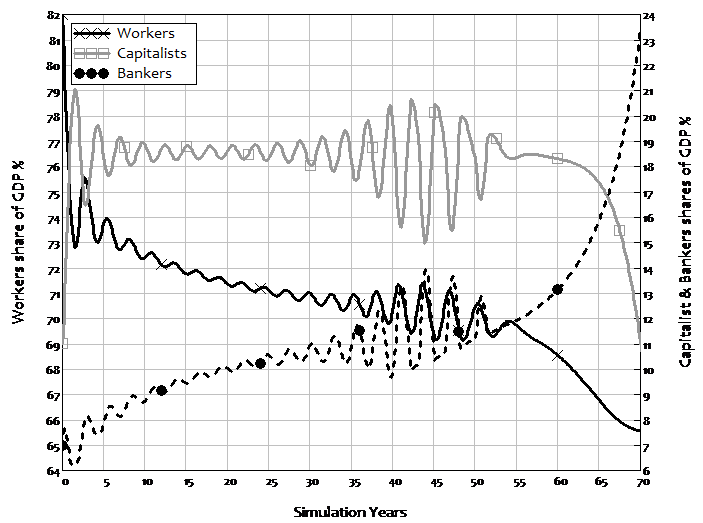
The model produces another prediction which has also become an empirical given: rising inequality. Workers’ share of GDP falls as the debt ratio rises, even though in this simple model, workers do no borrowing at all. If the debt ratio stabilises, then inequality stabilises too, as income shares reach positive equilibrium values. But if the debt ratio continues rising—as it does with a higher propensity to invest—then inequality keeps rising as well. Rising inequality is therefore not merely a “bad thing” in this model: it is also a prelude to a crisis.

The dynamics of rising inequality are more obvious in the next stage in the model’s development, which introduces prices and variable nominal interest rates. As debt rises over a number of cycles, a rising share going to bankers is offset by a smaller share going to workers, so that the capitalists share fluctuates but remains relatively constant over time. However, as wages and inflation are driven down, the compounding of debt ultimately overwhelms falling wages, and profit share collapses. Before this crisis ensues, the rising amount going to bankers in debt service is precisely offset by the declining share going to workers, so that profit share becomes effectively constant and the world appears utterly tranquil to capitalists—just before the system fails.

Figure 5: Rising inequality caused by rising debt

I built a version of this model in 1992, long before the “Great Moderation” was apparent. I had expected the model to generate a crisis, since I was attempting to model Minsky’s Financial Instability Hypothesis. But the moderation before the crisis was such a striking and totally unexpected phenomenon that I finished my paper by focusing on it, with what I thought was a nice rhetorical flourish:

From the perspective of economic theory and policy, this vision of a capitalist economy with finance requires us to go beyond that habit of mind which Keynes described so well, the excessive reliance on the (stable) recent past as a guide to the future. The chaotic dynamics explored in this paper should warn us against accepting a period of relative tranquility in a capitalist economy as anything other than a lull before the storm. (Keen, 1995b, p. 634. Emphasis added)

Though my model did predict that these phenomena of declining cycles in employment and inflation[1] and rising inequality would precede a crisis if one were to occur, I didn’t expect my rhetorical flourish to manifest itself in actual economic data. There were, I thought, too many differences between my simple, private-sector-only model and the complicated (as well as complex) real world for this to happen.

But it did.

[1] The wages share of output was a proxy for inflation in this simple model without price dynamics. The more complete model shown in Figure 5 explicitly includes inflation, and shows the same trend for inflation as found in the data.

[1] I’m sure some mainstream macroeconomists will dispute the use of this third definition, but I cover why it is essential in “The smoking gun of credit”. See also Kumhof and Jakab, (2015), which shows the dramatic impact of introducing private debt and endogenous money into a mainstream DSGE model.

[2] This compares to 7 variables, 49 parameters, and also random (stochastic) terms in the Smets-Wouters DSGE model mentioned earlier (see Romer, 2016, p. 12). See http://www.profstevekeen.com/crisis/models/ for the model’s equations and derivation. For the mathematical properties of this class of models, see Grasselli and Costa Lima (2012).

[3] Notably its linear behavioural rules and the absence of price dynamics means that the cycles are symmetrical—booms are as big as busts. These deficiencies are addressed in the model that generates Figure 5. There are issues also with these definitions, notably that of capital, which should not be ignored as they were after the “Cambridge Controversies” (Sraffa, 1960; Samuelson 1966). But these can be addressed by a disaggregation process, and are also made easier by acknowledging the role of energy in production. These topics are beyond the scope of this book, but I will address them in future more technical publications.

[4] “The source of financing most correlated with investment is long-term debt… debt plays a key role in accommodating year-by-year variation in investment”.

[1] The only limitation was that the shape had to be fitted by a polynomial—the sum of powers of x, x², x³, and so on: “every polynomial … is an excess demand function for a specified commodity in some n commodity economy” (Sonnenschein, 1972).