The Russian defeat of economic orthodoxy

Many armies have followed a triumphant march into Russia with an ignominious withdrawal. Orthodox economics is merely the latest invader to succumb to this dismal tradition. But this theory did more damage to the Russian Bear than most military invaders, writes Steve Keen, author of Debunking Economics: the naked emperor of the social sciences (Zed Books [US/UK] & Pluto Press).

Neoliberals were jubilant at the fall of the Berlin Wall. Not only had capitalism proved superior to communism, but the economic theory of the market economy had, it seemed, proved superior to Marxism. A task of transition did lie at “the end of history”—though not from capitalism to communism as Marx had expected, but from state socialism back to the market economy.

Such a transition was clearly necessary. In addition to the clear political and humanitarian failures of centralized Soviet regimes, economic growth under central planning had failed to maintain its initial promise. Once impressive performances gave way to stagnant economies producing dated goods, whereas the market economies of the West had grown more rapidly (if unevenly), and with far greater product innovation.

As the most prominent intellectual advocates for the free market over central planning, neoclassical economists presented themselves as the authorities for how this transition should occur. Above all else, they endorsed haste. In a typical statement, Murray Wolfson argued that

market systems are much more stable than most people who have been brought up in a command economy can imagine. The flexibility of market systems permits them to absorb a great deal of abuse and error that a rigidly planned system cannot endure. (Wolfson 1992, “Transition from a command economy: rational expectations and cold turkey”, Contemporary Policy Issues, Vol. 10, April: p. 42). [1]

The terms “abuse” and “error” were unfortunately prophetic—for the rapid transition imposed a great deal of abuse and error on the peoples of Eastern Europe. A decade later, incomes have collapsed, unemployment is at Great Depression levels, poverty is endemic. The transition has in general been not from Socialist to Capitalist, but from Socialist to Third World.

Wolfson is far from being a leading light of neoliberal economics. But his arguments in favour of a rapid transition are indicative of the naivety of those whom Joseph Stiglitz would eventually blame for abetting the theft and destruction of Russia’s wealth. Their key failing was a simplistic belief in the ability of market economies—even proto-market economies—to rapidly achieve equilibrium. This led them to recommend haste in the transition, and especially in privatization of state assets—a haste which effectively handed over state assets to those in a position to move quickly, the old Party appartachiks and organized crime.

Reading these pro-haste papers one decade after the transition debacle, one can take little comfort in realizing how different the outcome of this rapid transition was to the expectations economists held:

“Even though we favour rapid privatization, we doubt that privatization will produce immediate, large increases in productivity… Nonetheless, we believe that in order to enjoy these enormous long-term gains, it is necessary to proceed rapidly and comprehensively on creating a privately-owned, corporate-based economy in Eastern Europe” (Lipton & Sachs 1990: “Privatization in Eastern Europe: the case of Poland”, Brookings Papers on Economic Activity, 2: 1990, p. 295)

“The motivation for comprehensiveness and speed in introducing the reforms is clear cut. Such an approach vastly cuts the uncertainties facing the public with regard to the new ‘rules of the game’ in the economy. Rather than creating a lot of turmoil, uncertainty, internal inconsistencies, and political resistance, through a gradual introduction of new measures, the goal is to set in place clear incentives for the new economic system as rapidly as possible. As one wit has put it, if the British were to shift from left-hand-side drive to right-hand-side drive, should they do it gradually … say, by just shifting the trucks over to the other side of the road in the first round?” (Sachs, 1992. “The economic transformation of Eastern Europe: the case of Poland”, The American Economist, Vol. 36 No. 2: p. 5) [2]

It might be thought that, since speed was such a key aspect of the recommendations economists gave for the transition, they must have modeled the impact of slow versus fast transitions and shown that the latter were, in model terms at least, superior. But in fact the models economists took their guidance from completely ignored time: they were equilibrium models that presumed the system could rapidly move to a new equilibrium once disturbed.

The period of transition coincided with the peak influence of the concept of “rational expectations” in economic theory. This theory argues that a market economy is inhabited by “rational agents” who have, by some presumably evolutionary or iterative learning process, developed complete knowledge of the workings of the market economy and who can therefore confidently predict the future (at the very least, they know what will happen in response to any policy change by the government). The workings of the market economy happen to coincide with the behavior of a conventional neoclassical model, so that the economy is always in full employment equilibrium.

When this theory is put into a mathematical model, it results in a dynamic system known as a “saddle”, because the system dynamics are shaped like a horse’s saddle.

In conventional dynamic modeling, a saddle is an unstable system: the odds of the system being stable are the same as the odds of dropping a ball on to a real saddle and having it come to rest on the saddle, rather than falling off it. But if you were so lucky as to drop the ball precisely onto the saddle’s ridge, and it stayed on that ridge, it would ride up and down it for quite a while until it finally came to rest.

In rational expectations modeling, the saddle system that sensible dynamic models would say is unstable becomes stable but cyclical. The “rational agents” of the models all know the precise shape of the saddle, and jump onto its crest instantly from wherever they may have been displaced by a government policy change. Then the economy cycles up and down the ridge of the saddle, eventually coming to rest in full employment equilibrium once more. This is how devotees of rational expectations explain cycles, given their belief in the inherent equilibrium-seeking nature of a market economy: the system cycles up and down the sole stable path until coming to rest until it is once again disturbed.

These perspectives on individual behavior, the formation of expectations, and the behavior of a market economy, are dubious enough in their own right. Rational expectations “logic” is truly worthy of the moniker autistic, since it is based on a proposition that, if properly handled, negates its own predictions. This is the proposition that, as Muth put it:

Information is scarce, and the economic system generally does not waste it. (John Muth, “Rational Expectations and the Theory of Price Movements”: ) [3]

Since in neoclassical economics, scarcity is the basis of value, then information should according to this theory have a cost. If it has a cost, then agents should economize on its use—they will not use “all available information” but only the subset of information that they can afford, given their preferences for knowledge. Therefore individual agents will not know the full character of the economy, and most will certainly not know its “stable manifold”. Rational agents therefore cannot be expected to jump immediately to the equilibrium path of the economy unless they are irrational enough to expend the enormous amount of revenue that would be necessary to buy all the scarce information.

The foundations of “rational expectations” economics are thus internally inconsistent, and the fact that they were taken seriously in the first place is a clear sign of how truly autistic economic theory has become.

But if it was autistic to give this theory credence in the West, how much more so was it to apply this model to the behavior of people in an economic system in transition between central planning and market capitalism?

How can the “agents” in a transitional system develop a mental model of a market economy with which they predict the future behavior of the actual economy, if they have not previously lived in a market economy? Are we to presume instead that people can instantly develop the understanding of something as complex as a market economy—and are we to grace this belief with the adjective “rational”?

Lest this seem an overly harsh rhetorical flourish, consider the following discussion of how fast the transition should be from Wolfson’s 1992 paper. He begins with a statement that a sensible person might expect would lead towards the conclusion that people must be given time to learn how to react to market signals:

“Indeed, when government actions become so large that their effect on prices causes wide divergence from individual choices, one cannot determine what those choices would have been. As a result, no reliable guidelines exist for government choice. Even with the best of intentions, unlimited collective choice destroys the very information base for rational decisions.” (Wolfson 1992: 37). [1]

But instead, he immediately follows up this apparently sensible statement with the following proposition:

Central planners seemingly should at once resign their posts and close their offices. Their departure simply would signal the market to move immediately to equilibrium.” (Wolfson 1992: 37) [1]

What market? But oblivious to logical contradictions, he elaborates:

“For example, suppose the government were planning a gradual transition from a regime of administered prices to market prices to take place a year from now. What would happen 364 days hence? Obviously, people would refuse to make any but the most urgent transactions at the old prices, or an illegal market would immediately jump to the new prices. Those individuals who would have to sell their goods and services at a lower price on day 365 would find no legal customers on day 364. Similarly, those who would receive higher prices at day 364 would not sell legally on day 363, 362, 361, and so on. The economy would either come to a complete stop or would legally or illegally anticipate the future. In the face of rational and reasonably knowledgeable economic agents, delay invites disaster.” (Wolfson 1992: 37) [1]

“Rational and reasonably knowledgeable economic agents”? Where did they come from, and how did they acquire so profound a knowledge of the market system they have not as yet lived in that they can predict its behavior (and prices in it a year into the future) before they experience it? Yet presuming their existence and their intimate knowledge of the behavior of an economic system that does not yet exist, Wolfson advises that

A rational expectations conclusion is that quitting communism Cold Turkey is the only way to get from A to B. In practice, governments must make the national currency convertible and allow it to float on legal as well as black markets, abolish the system of subsidies and direct plans and quotas, close plants that cannot compete, come quickly to a privatization of industry even if some inequities result, strictly control the money supply, and allow goods and services to find their own price on national and international markets. (Wolfson 1992: 39; Wolfson does qualify his arguments with some concessions to reality, but in the end his recommendations are all for speed on the basis of a belief in the self-adjusting properties of the market economy) [1]

While there were significant differences in how the program of transition was implemented, in general this rapid and complete exposure of the once relatively closed economies of the East to the West was the rule. Away from the fantasies of rational expectations economics, what this rapid exposure to international competition did was give ex-socialist consumers instant access to Western goods, and expose Eastern European factories to open competition with their Western counterparts.

As Janos Kornai details so well [4, 5], the soft budget constraints of the Soviet system had resulted in “cashed up” consumers on the one hand, and technologically backward and shortage-afflicted factories on the other. The consumer financial surpluses, accumulated during the long wait between placing orders for consumer durables under the Soviet system and actually receiving the goods, were rapidly dissipated on Western consumer goods. The Eastern businesses, now forced to compete with technologically far superior Western firms, were rapidly destroyed, throwing their workers into unemployment. With accumulated buying power dissipated and freely floating currencies, exchange rates collapsed—for example, Romania’s Lei has gone from about 1,000 to the US dollar in 1993 to 32,000 to the dollar today.

A sensible dynamic analysis of the plight of the ex-socialist economies—one that really did take time into account—would have predicted this outcome from a too rapid transition. Even if the technological advantages of the market system over Soviet-style industrialization had amounted to just a one percentage difference per annum in productivity, the forty five year period of socialism would have given market economy firms a 55 per cent cost advantage over their socialist counterparts. And of course, the product development aspect of technological innovation had made far greater differences than this merely quantitative measure of costs—Western firms would have decimated socialist ones on product quality alone, even without a cost advantage.

A time-based analysis would therefore have supported a gradual transition, with substantial aid as well to assist Eastern factories to introduce modern production technology and process control methods. It should also have been obvious that for a market economy to develop, one needs the minimum distributive systems of a market: systems of wholesale and retail distribution, respect for written contracts, systems for consumer protection, laws of exchange—all things which take a substantial time to put in to place.

With the obscene haste with which the actual transition was implemented, the only non-market systems that could rapidly develop were those that were already in place in the preceding socialist system—the systems of organized crime that had always been there to lubricate the wheels of the shortage-afflicted Soviet system, just as market intrusions once permeated the feudal systems out of which capitalism itself evolved in Europe.

It is of course too late now to suggest any alternative path from socialism to the market for these no longer socialist economies. The new transition they must make is from a de-industrialized Third World state back to a developed one, and that transition will clearly take time.


[1] Wolfson, M. 1992 Transition from a Command Economy: Rational Expectations and Cold Turkey. Contemporary Economic Policy
10, 35.

[2] Sachs, J. 1992 The economic transformation of Eastern Europe: the case of Poland. Economics of Planning
25, 5-19. (doi:10.1007/BF00366287).

[3] Muth, J.F. 1961 Rational Expectations and the Theory of Price Movements. Econometrica
29, 315-335.

[4] Kornai, J. 1979 Resource-Constrained versus Demand-Constrained Systems. Econometrica
47, 801-819.

[5] Kornai, J. 1980 ‘Hard’ and ‘Soft’ Budget Constraint. Acta Oeconomica
25, 231-245. (doi:http://www.akademiai.com/content/119704/).


Economic failures of the IPCC process

The Intergovernmental Panel on Climate Change (IPCC) is the premier international body collating the scientific assessment of climate change, and proposals for mitigation. A joint creation of the United Nations agencies the World Meteorological Organization (WMO) and the United Nations Environment Programme (UNEP), it brings together scientists from myriad disciplines to assess and summarize the current research on climate change, collating knowledge that is then used to inform governments and politicians. The scientists work on a volunteer basis.

The IPCC relies upon its member governments and “Observers Organizations” to nominate its volunteer authors. This means that, subject to their willingness to volunteer, the most prestigious individuals specialising in climate change in each discipline become the authors of the relevant IPCC chapter for their discipline. They then undertake a review of the peer-reviewed literature in their field (and some non-peer-reviewed work, such as government reports) to distil the current state of knowledge about climate change in their discipline. A laborious review process is also followed, so the draft reports of the volunteer experts is reviewed by other experts in each field, to ensure conformity of the report with the discipline’s current perception of climate change. The emphasis upon producing reports which reflect the consensus within a discipline has resulted in numerous charges that the IPCC’s warnings are inherently too conservative (Herrando-Pérez et al., 2019, Brysse et al., 2013).

Figure 1: The IPCC’s graphic laying out the publication and review process behind its reports

But the main weaknesses with the IPCC’s methodology are firstly that, in economics, it exclusively selects Neoclassical economists, and secondly, because there is no built-in review of one discipline’s findings by another, the conclusions of these Neoclassical economists about the dangers of climate change are reviewed only by other Neoclassical economists. The economic sections of IPCC reports are therefore unchallenged by other disciplines who also contribute to the IPCC’s reports.

Given the extent to which economists dominate the formation of most government policies in almost all fields, and not just strictly economic policy (Fourcade et al., 2015, Hirschman and Berman, 2014, Christensen, 2018, Lazear, 2000), the otherwise acceptable process by which the IPCC collates human knowledge on climate change has critically weakened, rather than strengthened, human society’s response to climate change. This is because, commencing with “Nobel Laureate” (Mirowski, 2020) William Nordhaus, the economists who specialise on climate change have falsely trivialized the dangers that climate change poses to human civilization.

Nobel Oblige

In his 2018 Nobel Prize lecture, William Nordhaus described a trajectory that would lead to global temperatures peaking at 4°C above pre-industrial levels in 2145 as “optimal” (Nordhaus, 2018a, Slide 6) because, according to his calculations, the damages from climate change over time, plus the abatement costs over time, are minimised on this trajectory. He estimated the discounted cost of the economic damages from unabated climate change—which would see temperatures approach 6°C above pre-industrial levels by 2150—at $24 trillion, whereas the 4°C trajectory had damages of about $15 trillion and abatement costs of about $3 trillion. Trajectories with lower peak temperatures had higher abatement costs that overwhelmed the benefits (Nordhaus, 2018a, Slide 7). In a subsequent paper, Nordhaus claimed that even a 6°C increase would only reduce global income by only 7.9%, compared to what it would be in the complete absence of global warming.

This sanguine assessment of the costs of climate change contrasts starkly with the non-economic sections of IPCC reports. The recent Global Warming of 1.5°C Report, for example, predicted that 70% of insects and 40-60% of mammals would lose 50% or more of their range at 4.5°C (Warren et al., 2018, p. 792). Yet the economic components of IPCC reports concur with Nordhaus that damages from climate change will be slight: the Executive Summary of Chapter 10 of the 2014 Fifth Assessment, “Key Economic Sectors and Services”, opens with the declaration that:

For most economic sectors, the impact of climate change will be small relative to the impacts of other drivers (medium evidence, high agreement). Changes in population, age, income, technology, relative prices, lifestyle, regulation, governance, and many other aspects of socioeconomic development will have an impact on the supply and demand of economic goods and services that is large relative to the impact of climate change. (Arent et al., 2014a, p. 662)

How can such relatively small estimates of economic damages be reconciled with the large impacts that scientists expect on critical components of the biosphere? The answer is that they can’t, because the economic studies are not based on the scientific assessments of damage from climate change. Instead, the numerical estimates of the impact of climate change on GDP have been made up by economists themselves. I use the expression “made up” advisedly, because there is no more accurate way to characterise how Neoclassical economists have approached climate change. Before I explain how these spurious estimates were manufactured, it is useful to contrast them with some of the more easily understood dangerous consequences of a higher global average temperature.

The scientific assessment

Using Nordhaus’s sanguine prediction of a mere 7.9%
reduction in global income from a 6°C increase (Nordhaus, 2018b, p. 345) as a reference point, three of the most obvious threats of a 6°C warmer world are the impact of these temperatures on human physiology, on the survival of other animals, and on the structure of the Earth’s atmospheric circulation systems.

A critical feature of human physiology is our ability to dissipate internal heat by perspiration. To do so, the external air needs to be colder than our ideal body temperature of about 37°C, and dry enough to absorb our perspiration as well. This becomes impossible when the combination of heat and humidity, known as the “wet bulb temperature“, exceeds 35°C. Above this level, we are unable to dissipate the heat generated by our bodies, and the accumulated heat will kill a healthy individual within three hours. Scientists have estimated that a 3.8°C increase in the global average temperature would make Jakarta’s temperature and humidity combination permanently fatal for humans, while a 5.5°C increase would mean that even New York would experience 55 days per year when the combination of temperature and humidity would be deadly (Mora et al., 2017, Figure 4, p. 504).

Temperature also affects the viable range for all biological organisms on the planet. Scientists have estimated that a 4.5°C increase in global temperatures would reduce the area of the planet in which life could exist by 40% or more, with the decline in the liveable area of the planet ranging from a minimum of 30% for mammals to a maximum of 80% for insects (Warren et al., 2018, Figure 1, p. 792).

The Earth’s current climate has three major air circulation systems in each hemisphere: a “Hadley Cell” between the Equator and 30°, a mid-latitude cell between 30° and 60°, and a Polar cell between 60° and 90°. This structure is why there is such large differences in temperature between the tropics, temperate and arctic regions, and relatively small differences within each region. Scientists have modelled the stability of these cells and concluded that they could be tipped, by an average global temperature increase of 4.3°C or more, into a state with just one cell in the Northern Hemisphere—and an average Arctic temperature of 22.5°C. This abrupt transition (known as a bifurcation), sometime in the next century would disrupt agriculture, plant, animal and human life across the planet, and would occur far too quickly for any meaningful adaptation, by natural and human systems alike (Kypke et al., 2020, Figure 6 p. 399).

These three factors and many others, caused not only by industry’s CO2 emissions but also by the myriad other ways we damage the biosphere, would occur together, and interact with each other, at temperature levels of 4-6°C above pre-industrial levels. Nordhaus’s assertion that such devastating changes to the Earth’s climate would reduce global GDP by less than 8%, compared to a world without climate change (Nordhaus, 2018b, p. 345), is simply risible. How could he arrive at such an absurd conclusion?

In common with most of my peers in non-Neoclassical economics, I initially assumed that the answer was that he applied far too high a “discount rate” to future damages (Hickel, 2018). If you think that 99% of the economy would be destroyed in a century from now by the catastrophic effects of a 6°C increase in temperatures, but discount that back to today’s world at a rate of 7% p.a., you get the result that this collapse in future GDP is worth only 0.1% of today’s GDP—which is no big deal.

If this had been how Nordhaus had arrived at such low damage estimate, then the high discount rate could be challenged, but the rest of his analysis could potentially be sound. But our guess was wrong. Nordhaus explained why he used a high discount rate when he strongly criticised the lower discount rate used by the Stern Review (Stern, 2007). It was not to reduce future catastrophic damages to trivial levels now, but because, if he used a low discount rate, then:

the relatively small damages in the next two centuries get overwhelmed by the high damages over the centuries and millennia that follow 2200. (Nordhaus, 2007, p. 202. Emphasis added)

Relatively small damages in the next two centuries“? How on Earth did he reach that conclusion? I found out, to my disgust, that he and his colleagues ignored or distorted the work of scientists, and instead made up their own trivial estimates of the economic damage from climate change. I have spent fifty years of my life being a critic of Neoclassical economics. Neoclassical work on climate change is by far the lowest grade work that I have read in that half-century.

Reading Catastrophe and Seeing Utopia

I am accustomed to shaking my head in wonder at the capacity of Neoclassical economists to come up with ludicrous assumptions to jump over some logical impasse, like this gem by the developer of the Capital Assets Pricing Model, William Sharpe. After meticulously deriving a model of an individual “rational” investor, Sharpe then proceeded to model the entire market by assuming:

homogeneity of investor expectations: investors are assumed to agree on the prospects of various investments – the expected values, standard deviations and correlation coefficients described in Part II. (Sharpe, 1964, pp. 433-34, Fama and French, 2004, p. 26)

This is patently absurd. But at least Sharpe conceded as much, when he attempted to justify it via a clumsy rendition of Milton Friedman’s dodgy methodological defence of absurd assumptions (Friedman, 1953). Fama, who led the empirical defence of this theory (Fama, 1970, Fama and French, 1996, Fama and French, 2004), fitted it to actual stock market data, which for a time appeared to support the theory.

But in this work on climate change, Neoclassical economists have fitted their absurd-assumptions models to their own manifestly absurd made-up data. When they consulted scientists or referenced scientific literature, they frequently distorted the research or drowned the warnings of scientists with the blasé expectations of economists. This was nowhere more evident than in Nordhaus’s treatment of a key paper on the likelihood that global warming will trigger “tipping points” that cause runaway climate change, “Tipping elements in the Earth’s climate system” (Lenton et al., 2008).

Lenton’s paper considered whether there were large-scale elements of Earth’s climactic system which could be triggered into a qualitative change that would in turn rapidly alter the climate. He and his co-authors identified nine such systems (all but one of which—the Indian Monsoon—could be tipped by temperature increases alone), after applying the conditions that these systems had to be “subsystems of the Earth system that are at least subcontinental in scale” which could be “switched—under certain circumstances—into a qualitatively different state by small perturbations”. They excluded “systems in which any threshold appears inaccessible this century” (Lenton et al., 2008, pp. 1786-87).

If “Tipping elements” exist, and if they can be triggered by a temperature rise that can be expected from Global Warming this century, and if they would have drastic impacts upon the global climate, then the only prudent thing to do is to avoid such a temperature rise in the first place. If that rise occurs and a climactic element is tipped, it will unleash forces that will be far too large for human action to reverse. A qualitatively different climate would result, whose consequences for human civilisation cannot be predicted by extrapolating from what we know about our current climate.

Lenton and his co-authors identified two definite candidates for a tipping point this century—”Arctic sea-ice and the Greenland ice sheet”—and noted that “at least five other elements could surprise us by exhibiting a nearby tipping point” (Lenton et al., 2008, p. 1792) before 2100. They could not at the time specify a critical value for the temperature at which the decline in Arctic summer sea-ice would tip the Arctic from being a reflector of solar energy to an absorber, but noted that “a summer ice-loss threshold, if not already passed, may be very close and a transition could occur well within this century” (Lenton et al., 2008, p. 1789. Emphasis added).

Nordhaus “summarised” this research with the sentence:

“Their review finds no critical tipping elements with a time horizon less than 300 years until global temperatures have increased by at least 3°C” (Nordhaus, 2013a, p. 60)

This is a total fabrication. Lenton’s careful definition itself contradicts Nordhaus’s alleged summary, by explicitly excluding systems which could not be triggered this century. Nordhaus’s claim that they found no systems which could be triggered in the next three centuries is false: they identified at least two, and possibly seven (out of eight!), which could be—though the process of transiting from their current to final states could take several centuries. Nordhaus claimed that the minimum temperature rise that could trigger a “critical tipping element” was 3°C: they said that Arctic summer sea-ice could be triggered with a rise of as little as 0.5°C—a level we have already well and truly exceeded.

There are few—if any—scientific or economic issues that are more important than this. It deserves the closest possible attention. And yet, if an undergraduate student of mine had summarised this paper as Nordhaus did, I would have failed him. However, since I was reading the work of a “Nobel Prize winner”, rather than an unsatisfactory undergraduate, I found myself having to do forensic research to work how on Earth Nordhaus could have reached his interpretation of this paper—which explicitly warned against using “smooth projections of global change”, and which explicitly warned of a likely tipping point in the Arctic—as supporting him trivialising the significance of losing Arctic summer sea-ice, and using a “damage function” that ignored tipping points (see Table 1).

Table 1: The chasm between Lenton’s conclusion and Nordhaus’s interpretation of this research

The only feasible explanation for Nordhaus’s erroneous summary was a table by Lenton in a related publication (Richardson et al., 2011), which Nordhaus also referenced as a source for his interpretation (Nordhaus, 2013b, p. 334). Lenton described this table as “A simple ‘straw man’ example of tipping element risk assessment”. Each “tipping element” was given a point score in terms of likelihood of occurring this century (Low=1, Medium=1.5, Medium-High=2.5, and High=3) and relative impact on the climate over the next millennium (Low=1, Low-Medium=1.5, Medium=2, Medium-High=2.5, and High=3). A risk score was derived as the product of likelihood times impact. Arctic summer sea-ice had the lowest rating on impact (Low=1), but the highest in terms of likelihood (High=3), for an overall score of 3—see Table 2, which ranks these tipping elements in the descending order of importance that Nordhaus gave them in his table N.1 (Nordhaus, 2013b, p. 333).

Table 2: Based on Lenton’s Table “A simple ‘straw man’ example of tipping element risk assessment, by Timothy M. Lenton” in (Richardson et al., 2011, p. 186), and Nordhaus’s Table N-1, with his ranking of tipping elements used to sort the table (Nordhaus, 2013b, p. 333)

It appears that Nordhaus’s relative ranking was based primarily on Lenton’s “Impact” measure, since he ranked Arctic summer sea-ice as the lowest (one star in his Table N.1, or a low ranking of 3 in Table 2), below disrupting the Atlantic Thermohaline Circulation (THC) for example (two stars, or a medium ranking of 2), whereas Lenton ranked Arctic sea-ice above the THC in risk assessment terms (3 versus 2.5, where a higher score is worse) because of its much higher likelihood of occurring this century.

This may explain how Nordhaus came to classify losing the Arctic summer sea-ice as an event of low concern in climate change. But this is a false reading of Lenton’s table. As Lenton explained, “Impacts are considered in relative terms based on an initial subjective judgment (noting that most tipping-point impacts, if placed on an absolute scale compared to other climate eventualities, would be high)” (Richardson et al., 2011, p. 186. Emphasis added). In other words, while the impact of the loss of Arctic summer sea-ice was low compared to, for example, the impact of losing the Atlantic Thermohaline Circulation (THC), it was not low in any absolute sense: losing the Arctic’s summer sea-ice would have a significant qualitative impact on the climate. Nordhaus’s interpretation of Lenton’s “low” ranking as meaning that Arctic summer sea-ice was not of absolute importance to the climate—it was not “critical”, he alleged—is a fundamentally incorrect reading of Lenton’s research, as Lenton confirmed to me in personal correspondence (Keen and Lenton, 2020).

Nordhaus also misinterpreted the time ranges given (the “Transition Timescale” column in Table 2) as indicating that these tipping elements were not going to be triggered for that many years, when in fact they were an estimate of how long it would take from an initial triggering this century until the end of the transition process. The complete melting of the West Antarctic ice sheet might well take 300 years from its initial triggering, whereas the Arctic summer sea-ice could disappear over a period measured in decades rather than centuries. But the fate of the West Antarctic ice sheet would be decided this century, if we let increased CO2 levels drive up global temperature by 3°C or more—which we are well on track to do, and which we would reach on Nordhaus’s “optimum” trajectory by 2085.

In summary, Nordhaus read Lenton’s research as a climate change denier would, cherry picking it to find ways to support his preconception that climate change was insignificant. This was a consistent theme in Nordhaus’s treated scientific research on climate change, as evidenced by surveys he undertook of scientists in 1994 (Nordhaus, 1994), and scientific literature in 2017 (Nordhaus and Moffat, 2017).

Drowning Scientists with Economists

Nordhaus’s 1994 survey asked people from various academic backgrounds to give their estimates of the impact on GDP of three global warming scenarios, including a 3°C rise by 2090. The 2014 IPCC Report used this as one data point in Figure 10.1 (see Figure 2), claiming that a 3°C temperature rise would cause a 3.6% fall in GDP.

Nordhaus’s surveyed 19 people, 18 of whom fully complied, and one partially. Nordhaus described them as including 10 economists, 4 “other social scientists”, and 5 “natural scientists and engineers”, noting that eight of the economists come from “other subdisciplines of economics (those whose principal concerns lie outside environmental economics)” (Nordhaus, 1994, p. 48). This, ipso facto, should rule them out from taking part in this expert survey in the first place.

There was extensive disagreement between the relatively tiny cohort of actual scientists surveyed, and, in particular, the economists “whose principal concerns lie outside environmental economics”. As Nordhaus noted, “Natural scientists’ estimates [of the damages from climate change] were 20 to 30 times higher than mainstream economists'” (Nordhaus, 1994, p. 49). The average estimate by “Non-environmental economists” (Nordhaus, 1994, Figure 4, p. 49) of the damages to GDP a 3°C rise by 2090 was 0.4% of GDP; the average for natural scientists was 12.3%, and this was with one of them refusing to answer Nordhaus’s key questions:

“I must tell you that I marvel that economists are willing to make quantitative estimates of economic consequences of climate change where the only measures available are estimates of global surface average increases in temperature. As [one] who has spent his career worrying about the vagaries of the dynamics of the atmosphere, I marvel that they can translate a single global number, an extremely poor surrogate for a description of the climatic conditions, into quantitative estimates of impacts of global economic conditions.” (Nordhaus, 1994, pp. 50-51)

Comments from economists lay at the other end of the spectrum from this self-absented scientist. Because they had a strong belief in the ability of human economies to adapt, they could not imagine that climate change could do significant damage to the economy, whatever it might do to the biosphere itself:

There is a clear difference in outlook among the respondents, depending on their assumptions about the ability of society to adapt to climatic changes. One was concerned that society’s response to the approaching millennium would be akin to that prevalent during the Dark Ages, whereas another respondent held that the degree of adaptability of human economies is so high that for most of the scenarios the impact of global warming would be “essentially zero”. (Nordhaus, 1994, pp. 48-49. Emphasis added)

Given this extreme divergence of opinion between economists and scientists, one might expect that Nordhaus’s next survey would examine the reasons for it. In fact, the opposite applied: his methodology excluded non-economists entirely.

Rather than a survey of experts, this was a literature survey (Nordhaus and Moffat, 2017). He and his co-author searched for relevant articles using the string “”(damage OR impact) AND climate AND cost” (Nordhaus and Moffat, 2017, p. 7), which is reasonable, if too broad (as they admit in the paper).

The key
flaw in this research was where they looked: they executed their search string in Google, which returned 64 million results, Google Scholar, which returned 2.8 million, and the economics-specific database Econlit, which returned just 1700 studies. On the grounds that there were too many results in Google and Google Scholar, they ignored those results, and simply surveyed the 1700 articles in Econlit (Nordhaus and Moffat, 2017, p. 7). These are, almost exclusively, articles written by economists. They did not search a comparable science database like ProQuest Science Journals, where the same too-broad search string (on January 11th 2021) returned 60,315 peer-reviewed full-text articles, and a narrower search string “damage AND climate AND gdp” returned a manageable 2,721 hits.

There is therefore no significant science-based content in the papers that generated the “data” on which IPCC economists concluded that “the impact of climate change will be small relative to the impacts of other drivers” (Arent et al., 2014a, p. 662). All of the pairs of numbers in Figure 2 were generated by economists, and all but one predict an extremely small impact on GDP from global warming, of a less than 3% fall in GDP from temperature rises of up to 3°C (or a 6% fall for a 5.5°C rise), compared to what GDP would be in the complete absence of climate change.

Figure 2: IPCC economic estimates of damages to GDP from global warming (Arent et al., 2014a, p. 690)

These numbers were generated in two main ways, which the IPCC report described as “Enumeration” and “Statistical” (Arent et al., 2014b, Table SM10.2, p. SM10-4). Enumeration added up estimates of damages to industries from climate change, under the assumption that only activities exposed to the weather would be affected; the “statistical” method used the weak correlation between average temperature and average income today as a proxy for the impact of climate change over time.

Equating Climate with Weather

Nordhaus’s first predictions of the economic consequences of climate change in a refereed journal—the Economic Journal—came in 1991. This paper, entitled “To Slow or Not to Slow: The Economics of The Greenhouse Effect” (Nordhaus, 1991) contained the seeds of all his future work on climate change. He equated climate change over time, due to dramatically increasing the amount of solar radiation retained in the biosphere as heat by increased greenhouse gases, with the geographic variation of today’s climate across the globe:

human societies thrive in a wide variety of climatic zones. For the bulk of economic activity, non-climate variables like labour skills, access to markets, or technology swamp climatic considerations in determining economic efficiency. (Nordhaus, 1991, p. 930)

He assumed that climate change would only affect economic activities that were directly exposed to the weather:

The most sensitive sectors are likely to be those, such as agriculture and forestry, in which output depends in a significant way upon climatic variables… Our estimate is that approximately 3% of United States national output is produced in highly sensitive sectors, another 10% in moderately sensitive sectors, and about 87 % in sectors that are negligibly affected by climate change. (Nordhaus, 1991, Table 5, p. 930. Emphasis added)

Table 3: Extract from Nordhaus’s breakdown of economic activity by vulnerability to climatic change (Nordhaus, 1991, p. 931)

Using these beliefs, he derived trivial estimates for the impact of climate change on the economy:

damage from a 3°C warming is likely to be around ¼% of national income in United States … We might raise the number to around 1% of total global income to allow for these unmeasured and unquantifiable factors, although such an adjustment is purely ad hoc… my hunch is that the overall impact upon human activity is unlikely to be larger than 2% of total output. (Nordhaus, 1991, p. 933)

All subsequent papers by Neoclassical climate-change economists replicated the assumption that any activity not directly exposed to the weather would be immune from climate change. The 2014 IPCC Report restated it as a “Frequently Asked Question”:

FAQ 10.3 | Are other economic sectors vulnerable to climate change too?

Economic activities such as agriculture, forestry, fisheries, and mining are exposed to the weather and thus vulnerable to climate change. Other economic activities, such as manufacturing and services, largely take place in controlled environments and are not really exposed to climate change. (Arent et al., 2014a, p. 688. Emphasis added)

Equating Time with Space

Nordhaus’s colleague Robert Mendelsohn (Mendelsohn et al., 1994, Mendelsohn et al., 2000) used Nordhaus’s assumption that today’s climate and GDP data was relevant to climate change to invent another way to predict the impact of global warming from today’s data:

An alternative approach … can be called the statistical approach. It is based on direct estimates of the welfare impacts, using observed variations (across space within a single country) in prices and expenditures to discern the effect of climate. Mendelsohn assumes that the observed variation of economic activity with climate over space holds over time as well; and uses climate models to estimate the future effect of climate change. (Tol, 2009, p. 32. Emphasis added)

This method of generating numbers takes average temperature data and per capita income data, and uses the weak correlation between them to allege that climate change will be relatively trivial. Figure 3 shows temperature and per capita income for the contiguous United States on a State-by-State basis (“Gross State Product per capita”, or GSPPC).

Figure 3: Correlation of temperature and USA Gross State Product per capita

There is no real pattern, but a quadratic can be fitted to the data as shown, with a low correlation coefficient of 0.31. In statistical terms, this means that this function has terrible predictive power. For example, it predicts that States which are 4°C hotter or colder than the USA average will have a GSPPC that is 5% lower. But the states that are between 3.5°C and 4.5°C above or below the USA’s average temperatures include New York at 30% above the average, and Arkansas at 29% below. If you were trying to win a game of Trivial Pursuit, you wouldn’t use this function to supply your answers on US GSP per capita today.

Trivial estimates of serious damages

And yet Nordhaus uses a quadratic, derived from data much like that in Figure 3, but with an even smaller coefficient, to “predict” the impact of Global Warming on “Gross Global Product” (GGP). The equation of the quadratic in Figure 3 is . Nordhaus’s “damage function”, in the latest version of his global warming model DICE (for “Dynamic Integrated Climate and Economics”), is :

The parameter used in the model was an equation with a parameter of 0.227 percent loss in global income per degrees Celsius squared with no linear term. This leads to a damage of 2.0 percent of income at 3°C, and 7.9 percent of global income at a global temperature rise of 6°C. (Nordhaus, 2018b, p. 345)

These predictions are absurd. A 3°C increase could trigger, and a
6°C increase would trigger, every “tipping element” shown in Table 2. The Earth would have a climate unlike anything our species has experienced in its existence, and the Earth would transition to it hundreds of times faster than it has in any previous naturally-driven global warming event (McNeall et al., 2011). The Tropics and much of the globe’s temperate zone would be uninhabitable by humans and most other life forms. And yet Nordhaus thinks it would only reduce the global economy by just 8%?

Comically, Nordhaus’s damage function is symmetrical—it predicts the same damages from a fall in temperature as for an equivalent rise. It therefore predicts that a 6°C fall in global temperature would also reduce GGP by just 7.9% (see Figure 3). Unlike global warming, we do know what the world was like when the temperature was 6°C below 20th century levels: that was the average temperature of the planet during the last Ice Age (Tierney et al., 2020), which ended about 20,000 years ago. At the time, all of America north of New York, and of Europe north of Berlin, was beneath a kilometre of ice. The thought that a transition to such a climate in just over a century would cause global production to fall by less than 8% is laughable.

Again, I found myself in the position of a forensic detective, trying to work out how on Earth could otherwise intelligent people come to believe that climate change would only affect industries that are directly exposed to the weather, and that the correlation between climate today and economic output today across the globe could be used to predict the impact of global warming on the economy? The only explanation that made sense is that these economists were mistaking the weather for the climate. Ironically, given the calibre of Nordhaus’s later contributions, he gave a reasonable, if statistically-oriented, explanation of the difference between weather and climate in an early paper:

When we refer to climate, we usually are thinking of the average of characteristics of the atmosphere at different points of the earth, including the variances such as the diurnal and annual cycle. The important characteristics for man’s activities are temperature, precipitation, snow cover, winds and so forth. A more precise representation of the climate would be as a dynamic, stochastic system of equations. The probability distributions of the atmospheric characteristics is what we mean by climate, while a particular realization of that stochastic process is what we call the weather. (Nordhaus, 1976, p. 2)

This “probability distribution”, as we experience it at any given location on Earth, is affected by the amount of energy in the biosphere, which varies in three primary ways:

  1. Variations in the amount of the energy from the Sun that reaches the Earth;
  2. Variations in the amount of this energy retained by greenhouse gases; and
  3. Variations caused by differences in location on the planet—primarily, differences in distance from the Equator, altitude above sea level, and distance from oceans.

The first factor varies, via cyclical variations in the Earth’s orbit, over time measured in thousands of years, and via long-term trends in the Sun’s evolution, measured in billions of years. Neither of these are relevant in the timeframe of global warming. Given the Earth’s orbit, and how much its surface reflects solar radiation, then in the absence of the second factor—greenhouse gases—the average temperature of the atmosphere would be minus 18°C (Hay, 2014, p. 30, Galimov, 2017).

The second is what is at issue with global warming. If the Earth’s atmosphere captured and re-radiated all the infra-red energy that the planet’s surface reflects back into space (as a relatively dark body, the Earth absorbs high-frequency light and ultra-violet energy from the Sun, and reflects back low-frequency infra-red energy), then the average temperature of the atmosphere would be 29.5°C. With only naturally-occurring greenhouse gases, the average temperature of the planet at present would be 15°C. Human industrial activity is adding to this retention of solar energy, primarily by generating additional CO2 from burning fossil fuels.

The third, geographic factor is what is captured by the data shown in Figure 3—and this has nothing to do with global warming. And yet this data, plus the belief that only industries which are exposed to the weather will be affected by global warming, is what underpins Nordhaus’s “damage function” (and similar constructs by his fellow Neoclassical climate change economists) with its trivial forecasts for economic damage from climate change.

One thing that Figure 3 does establish is that wide variations in temperature within one country today are associated with relatively small differences in income today. The range of average temperatures shown there is 16.8°C, from 4.7°C for North Dakota to 21.5°C for Florida. However, the two States had very similar Gross State Products per capita in 2000 ($26,700 versus $26,000). This cannot be used to argue that, therefore, a huge change in global average temperatures due to global warming will have only a small effect on income—but that is precisely how Neoclassical economists have used this data.

That is evident in their predictions, but it helps to also have verbal confirmation of the disconnect between what economists think of climate change, and what it really is. The following statements were made on Twitter by the prominent Neoclassical climate change economist Richard Tol. Tol was one of the two lead co-authors of the economic sections of the 2014 IPCC report on climate change (Arent et al., 2014a), the developer of FUND (“Climate Framework for Uncertainty, Negotiation and Distribution“), one of “Integrated Assessment models” (IAMs) used to supposedly estimate the impact of climate change on the economy, and editor of the academic journal Energy Economics. However, his arguments are those one would with associate with an ignorant troll, not an influential economist in the theory and practice of climate change.

In the first tweet, he concludes that climate change is not a problem, because US States with vastly different temperatures today have similar incomes today:

10K is less than the temperature distance between Alaska and Maryland (about equally rich), or between Iowa and Florida (about equally rich). Climate is not a primary driver of income. https://twitter.com/RichardTol/status/1140591420144869381?s=20

In the second, he concludes that global warming can’t be a problem, because it is expected to increase temperatures by a small amount compared to the daily temperature variation for any one location on Earth—which averages about 14°C for the continental USA (Qu et al., 2014):

People thrive in a wide range of climates. The projected climate change is small relative to the diurnal cycle. It is therefore rather peculiar to conclude that climate change will be disastrous. Those who claim so have been unable to explain why. https://twitter.com/RichardTol/status/1313182006310731776?s=20

My personal experience of responding to delusional beliefs like these reminds me of the aphorism widely attributed to George Bernard Shaw, that “he who wrestles with a hog must expect to be spattered with filth, whether he is vanquished or not”. In contrast, this is how a key scientific paper (Im et al., 2017`) summarised what a world 4°C warmer—let alone 10°C-14°C warmer—would mean for the over 2 billion human inhabitants of South Asia:

Human exposure to TW [wet bulb temperatures] of around 35°C for even a few hours will result in death even for the fittest of humans under shaded, well-ventilated conditions… TWmax is projected to exceed the survivability threshold … under the RCP8.5 scenario by the end of the century over most of South Asia, including the Ganges river valley, northeastern India, Bangladesh, the eastern coast of India, Chota Nagpur Plateau, northern Sri Lanka, and the Indus valley of Pakistan. (Im et al., 2017, p. 4)

The failure of peer review

There is one generic defence of the failure of the referees of economic journals to identify this work as effectively fraudulent. Academics are not paid to referee, and the time they are supposedly allotted to do refereeing has been largely eliminated by the efficiency drives that politicians and the managerial class of University administrators have forced upon them. So refereeing is not done as professionally as the image of “peer reviewed research” implies. Refereeing is also a far lower standard than replication. To referee a paper, all a referee has to do is read it and pass judgment. To replicate, you actually have to independently reproduce the results claimed in the paper.

That said, there is no excuse for referees approving for publication papers that, for example, make the critical and absurd assumption that 87% of GDP will be unaffected by climate change, because it happens indoors (Nordhaus, 1991, p. 930). Here, the guilty party is not Nordhaus alone, but the entire edifice of Neoclassical economics. Only Neoclassical economists, who in general have what Paul Romer described as a “noncommittal relationship with the truth” (Romer, 2016, p. 5), would recommend publication of papers that make critical assumptions that are so obviously false.

As I detail in Debunking Economics (Keen, 2011), Neoclassical economics is riddled with false assumptions, because numerous theoretical and empirical requirements of the underlying theory have been proven to be false. Rather than accepting that their initial beliefs were wrong, and then abandoning these beliefs to develop a richer, more complex theory, Neoclassical economists have clung to those beliefs by adding patently absurd assumptions to hide the contrary proofs.

This practice is defended by describing such assumptions as “simplifying”, but that a false description. A simplifying assumption is something that, if it is false, complicates the analysis a great deal, but changes the result only marginally. For example, Galileo’s demonstration that dense bodies fall at the same speed, regardless of their weight, effectively assumed no air resistance. Taking air resistance into account would have resulted in a vastly more complicated demonstration, but no significant change in the result.

On the other hand, the type of assumption that Neoclassical economists defend as “simplifying” is frequently critical to the conclusions drawn from the model: if the assumption is false, then so are the conclusions (Musgrave, 1990). Such assumptions abound in Neoclassical economics, so much so that economists have convinced themselves that it is invalid to criticise a theory on the grounds that its assumptions are unrealistic:

To put this point less paradoxically, the relevant question to ask about the “assumptions” of a theory is not whether they are descriptively “realistic”, for they never are, but whether they are sufficiently good approximations for the purpose in hand. And this question can be answered only by seeing whether the theory works, which means whether it yields sufficiently accurate predictions. (Friedman, 1953, p. 153)

This, as Alan Musgrave explained, is nonsense (Musgrave, 1981). However, because they accept Friedman’s dodgy methodology, Neoclassical referees regularly recommend the publication of papers in which assumptions are made that are patently false, if those papers support Neoclassical beliefs. To such referees, Nordhaus’s assumption that “87% [of United States national output is produced] in sectors that are negligibly affected by climate change” (Nordhaus, 1991, p. 930) was just a “simplifying assumption”, which could not be challenged.

This methodological fallacy is dangerous enough with standard economic issues. But with climate change, it is existentially so. When the theory is proven wrong by the failure of its predictions, the consequences of this failure will be both catastrophic and irreversible. As DeCanio eloquently put it, waiting until we know that Neoclassical economists are wrong on climate change “amounts to conducting a one-time, irreversible experiment of unknown outcome with the habitability of the entire planet” (DeCanio, 2003, p. 3).

Conclusion

Neoclassical economics has dominated economics for 150 years, which has given it the advantage of incumbency over its rivals—so much so that most people in authority, journalists, University students, and the general public, think that Neoclassical economics is economics. When it is criticised, even by other economists like myself (Keen, 2011), the public is unlikely to hear the criticisms in the first place, and likely to regard them as coming from cranks if they do. Q-Anon aside, we trust those ordained as experts in their own fields.

This trust is a characteristic of human society which is utterly justified in the complex societies in which we live. Deference to expertise is a necessary feature of life in a complex world. However, with economics, this justifiable deference has helped entrench a fundamentally unscientific school of thought, and has made progress in economics virtually impossible.

I believed, before the Global Financial Crisis, that the only way economics could be shifted would be by its failure to predict a serious economic crisis. But the transient nature of economic crises—especially in the face of governments determined not to let capitalism fail on their watch—meant that economic theory scraped through that crisis relatively unscathed. That may all change in the next decade, because our trust in expertise has meant that, though scientists led the study of climate change, we have let Neoclassical economists determine our policy response.

Most politicians have studied some economics. Few have studied science, and they are therefore unable to read the science-based parts of the IPCC Reports. Most of their advisers—who actually read the reports for the politicians—are also trained in economics, rather than the sciences. Most political debate is about matters of economics, rather than science. The end result of all this is that, though scientists have led the study of climate change itself, economists have dominated public policy towards it. As Stephen De Canio put it in 2003:

it is undeniably the case that economic arguments, claims, and calculations have been the dominant influence on the public political debate on climate policy in the United States and around the world… It is an open question whether the economic arguments were the cause or only an ex-post justification of the decisions made … but there is no doubt that economists have claimed that their calculations should dictate the proper course of action. (DeCanio, 2003, p. 4)

Because these economists, starting with William Nordhaus, trivialised the dangers of climate change, the policy response to climate change has also been trivial. Human civilisation may well not survive Neoclassical economics. It’s time it was eliminated, before it eliminates us.

References

ARENT, D. J., TOL, R. S. J., FAUST, E., HELLA, J. P., KUMAR, S., STRZEPEK, K. M., TÓTH, F. L. & YAN, D. 2014a. Key economic sectors and services. In: FIELD, C. B., BARROS, V. R., DOKKEN, D. J., MACH, K. J., MASTRANDREA, M. D., BILIR, T. E., CHATTERJEE, M., EBI, K. L., ESTRADA, Y. O., GENOVA, R. C., GIRMA, B., KISSEL, E. S., LEVY, A. N., MACCRACKEN, S., MASTRANDREA, P. R. & WHITE, L. L. (eds.) Climate Change 2014: Impacts, Adaptation, and Vulnerability. Part A: Global and Sectoral Aspects. Contribution of Working Group II to the Fifth Assessment Report of the Intergovernmental Panel on Climate Change. Cambridge, United Kingdom: Cambridge University Press.

ARENT, D. J., TOL, R. S. J., FAUST, E., HELLA, J. P., KUMAR, S., STRZEPEK, K. M., TÓTH, F. L. & YAN, D. 2014b. Key economic sectors and services – supplementary material. In: FIELD, C. B., BARROS, V. R., DOKKEN, D. J., MACH, K. J., MASTRANDREA, M. D., BILIR, T. E., CHATTERJEE, M., EBI, K. L., ESTRADA, Y. O., GENOVA, R. C., GIRMA, B., KISSEL, E. S., LEVY, A. N., MACCRACKEN, S., MASTRANDREA, P. R. & WHITE, L. L. (eds.) Climate Change 2014: Impacts, Adaptation, and Vulnerability. Part A: Global and Sectoral Aspects. Contribution of Working Group II to the Fifth Assessment Report of the Intergovernmental Panel on Climate Change Geneva: IPCC.

BRYSSE, K., ORESKES, N., O’REILLY, J. & OPPENHEIMER, M. 2013. Climate change prediction: Erring on the side of least drama? Global environmental change, 23, 327-337.

CHRISTENSEN, J. 2018. Economic knowledge and the scientization of policy advice. Policy Sciences, 51, 291-311.

DECANIO, S. J. 2003. Economic models of climate change : a critique, New York, Palgrave Macmillan.

FAMA, E. F. 1970. Efficient Capital Markets: A Review of Theory and Empirical Work. The Journal of Finance, 25, 383-417.

FAMA, E. F. & FRENCH, K. R. 1996. The CAPM Is Wanted, Dead or Alive. Journal of Finance, 51, 1947-1958.

FAMA, E. F. & FRENCH, K. R. 2004. The Capital Asset Pricing Model: Theory and Evidence. The Journal of Economic Perspectives, 18, 25-46.

FOURCADE, M., OLLION, E. & ALGAN, Y. 2015. The superiority of economists. Journal of Economic Perspectives, 29, 89-114.

FRIEDMAN, M. 1953. The Methodology of Positive Economics. Essays in positive economics. Chicago: University of Chicago Press.

GALIMOV, E. M. 2017. Role of low solar luminosity in the history of the biosphere. Geochemistry international, 55, 401-417.

GOODWIN, R. M. 1967. A growth cycle. In: FEINSTEIN, C. H. (ed.) Socialism, Capitalism and Economic Growth. Cambridge: Cambridge University Press.

GRASSELLI, M. R. & MAHESHWARI, A. 2017. A comment on ‘Testing Goodwin: growth cycles in ten OECD countries’. Cambridge Journal of Economics, 41, 1761-1766.

HARVIE, D. 2000. Testing Goodwin: Growth Cycles in Ten OECD Countries. Cambridge Journal of Economics, 24, 349-376.

HAY, W. W. 2014. The accelerating rate of global change. Rendiconti Lincei, 25, 29-48.

HERRANDO-PÉREZ, S., BRADSHAW, C. J. A., LEWANDOWSKY, S. & VIEITES, D. R. 2019. Statistical Language Backs Conservatism in Climate-Change Assessments. Bioscience, 69, 209-219.

HICKEL, J. 2018. The Nobel prize for climate catastrophe. Foreign Policy.

HIRSCHMAN, D. & BERMAN, E. P. 2014. Do economists make policies? On the political effects of economics1. Socio-Economic Review, 12, 779-811.

IM, E.-S., PAL, J. S. & ELTAHIR, E. A. B. 2017. Deadly heat waves projected in the densely populated agricultural regions of South Asia. Science advances, 3, e1603322-e1603322.

KEEN, S. 2011. Debunking economics: The naked emperor dethroned?, London, Zed Books.

KEEN, S. & LENTON, T. June 11th 2020 2020. RE: Draft paper on Nordhaus et al which cites you. Type to LENTON, T.

KYPKE, K. L., LANGFORD, W. F. & WILLMS, A. R. 2020. Anthropocene climate bifurcation. Nonlinear processes in geophysics, 27, 391-409.

LAZEAR, E. P. 2000. Economic Imperialism. Quarterly Journal of Economics, 115, 99-146.

LENTON, T. M., HELD, H., KRIEGLER, E., HALL, J. W., LUCHT, W., RAHMSTORF, S. & SCHELLNHUBER, H. J. 2008. Tipping elements in the Earth’s climate system. Proceedings of the National Academy of Sciences, 105, 1786-1793.

MCNEALL, D., HALLORAN, P. R., GOOD, P. & BETTS, R. A. 2011. Analyzing abrupt and nonlinear climate changes and their impacts. Wiley Interdisciplinary Reviews: Climate Change, 2, 663-686.

MENDELSOHN, R., NORDHAUS, W. D. & SHAW, D. 1994. The Impact of Global Warming on Agriculture: A Ricardian Analysis. The American Economic Review, 84, 753-771.

MENDELSOHN, R., SCHLESINGER, M. & WILLIAMS, L. 2000. Comparing impacts across climate models. Integrated Assessment, 1, 37-48.

MIROWSKI, P. 2020. The Neoliberal Ersatz Nobel Prize. In: PLEHWE, D., SLOBODIAN, Q. & MIROWSKI, P. (eds.) Nine Lives of Neoliberalism. London: Verso.

MORA, C., BÉNÉDICTE, D., IAIN, R. C., FARRAH, E. P., ROLLAN, C. G., CORAL R, B., CHELSIE, W. W. C., BONNIE, S. D., EMILY, T. J., LEO, V. L., MATTHEW, P. L., MARIE, M. M., ALESSANDRA, G. S., HAN, T., THOMAS, W. G., LISA, R. L., ED, H. & CLAY, T. 2017. Global risk of deadly heat. Nature Climate Change, 7.

MUSGRAVE, A. 1981. ‘Unreal Assumptions’ in Economic Theory: The F‐Twist Untwisted. Kyklos (Basel), 34, 377-387.

MUSGRAVE, A. 1990. ‘Unreal Assumptions’ in Economic Theory: The F-Twist Untwisted. In: WOOD, J. C. & WOODS, R. N. (eds.) Milton Friedman: Critical assessments. Volume 3. London and New York: Routledge.

NORDHAUS, W. 1976. Strategies for the Control of Carbon Dioxide. Cowles Foundation Discussion Paper.

NORDHAUS, W. 1994. Expert Opinion on Climate Change. American Scientist, 82, 45–51.

NORDHAUS, W. 2007. Critical Assumptions in the Stern Review on Climate Change. Science, 317, 201-202.

NORDHAUS, W. 2013a. The Climate Casino: Risk, Uncertainty, and Economics for a Warming World, New Haven, CT, Yale University Press.

NORDHAUS, W. 2013b. NOTES. The Climate Casino. Yale University Press.

NORDHAUS, W. 2018a. Nobel Lecture in Economic Sciences. Climate Change: The Ultimate Challenge for Economics [Online]. Stockholm: Nobel Prize in Economics Committee. Available: https://www.nobelprize.org/uploads/2018/10/nordhaus-slides.pdf [Accessed].

NORDHAUS, W. 2018b. Projections and Uncertainties about Climate Change in an Era of Minimal Climate Policies. American Economic Journal: Economic Policy, 10, 333–360.

NORDHAUS, W. & SZTORC, P. 2013. DICE 2013R: Introduction and User’s Manual.

NORDHAUS, W. D. 1980. Thinking About Carbon Dioxide: Theoretical and Empirical Aspects of Optimal Control Strategies. Cowles Foundation Discussion Paper.

NORDHAUS, W. D. 1991. To Slow or Not to Slow: The Economics of The Greenhouse Effect. The Economic Journal, 101, 920-937.

NORDHAUS, W. D. & MOFFAT, A. 2017. A Survey Of Global Impacts Of Climate Change: Replication, Survey Methods, And A Statistical Analysis. New Haven, Connecticut: Cowles Foundation.

QU, M., WAN, J. & HAO, X. 2014. Analysis of diurnal air temperature range change in the continental United States. Weather and Climate Extremes, 4, 86-95.

RICHARDSON, K., STEFFEN, W. & LIVERMAN, D. 2011. Climate Change: Global Risks, Challenges and Decisions, Cambridge, Cambridge University Press.

ROMER, P. 2016. The Trouble with Macroeconomics. Available from: https://paulromer.net/trouble-with-macroeconomics-update/WP-Trouble.pdf.

SHARPE, W. F. 1964. Capital Asset Prices: A Theory of Market Equilibrium under Conditions of Risk. The Journal of Finance, 19, 425-442.

STERN, N. 2007. The Economics of Climate Change : The Stern Review / Nicholas Stern, Cambridge : Cambridge University Press.

TIERNEY, J. E., ZHU, J., KING, J., MALEVICH, S. B., HAKIM, G. J. & POULSEN, C. J. 2020. Glacial cooling and climate sensitivity revisited. Nature (London), 584, 569-573.

TOL, R. S. J. 2009. The Economic Effects of Climate Change. The Journal of Economic Perspectives, 23, 29–51.

WARREN, R., PRICE, J., GRAHAM, E., FORSTENHAEUSLER, N. & VANDERWAL, J. 2018. The projected effect on insects, vertebrates, and plants of limiting global warming to 1.5°C rather than 2°C. Science, 360, 791-795.


A 2020 Retrospective: Looking Back in Foresight

I made the macabre joke at the end of my post on losing David Graeber, that “Now we know why we speak of 20:20 vision, and 20:20 hindsight. We thought it was an ophthalmologist’s crazy numbering system. In fact, it was a warning from a time traveler.” That year is about to pass, and we’ll soon look back on 2020 in hindsight—as we once did on 1920, when the Spanish Flu ended.

Will we be any the wiser? I unfortunately expect that the wish to see this year in the rear vision mirror will translate into a wish to “return to normal”, where normal is defined as “what was happening before 2020”. However, that pre-2020 normal itself was based on so many unsustainable trends—most significantly of all, the unsustainable trend of human exploitation of the biosphere. 2020 will probably be looked back upon as the year in which the unsustainability of those trends was first made apparent by Covid-19. But we humans are likely not to learn that lesson, given our desire to escape the pain this year has caused.

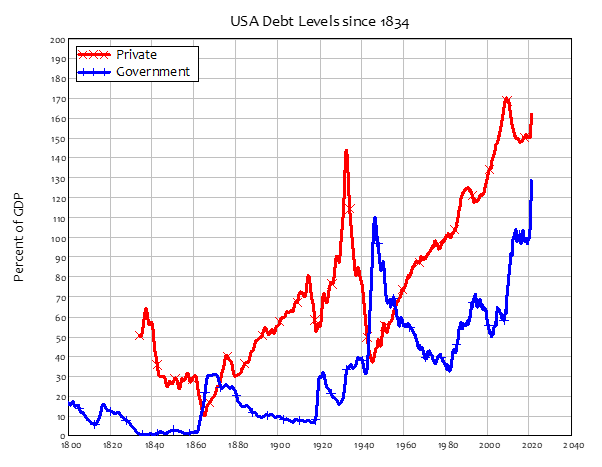
Some Twitter correspondents have wondered whether The Roaring Twenties were a similar response, after the privations forced upon America by the Spanish Flu. I think there’s wisdom in that thought, and I do expect we’ll attempt likewise. But we will be bereft of the low levels of private debt, and low relative levels of the stock market, that made that euphoria possible in 1920.

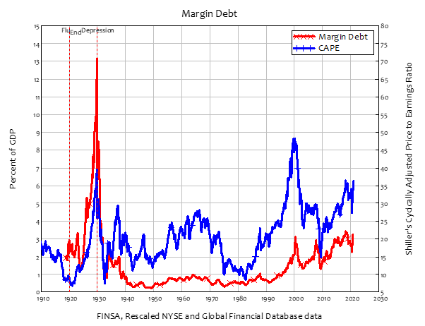
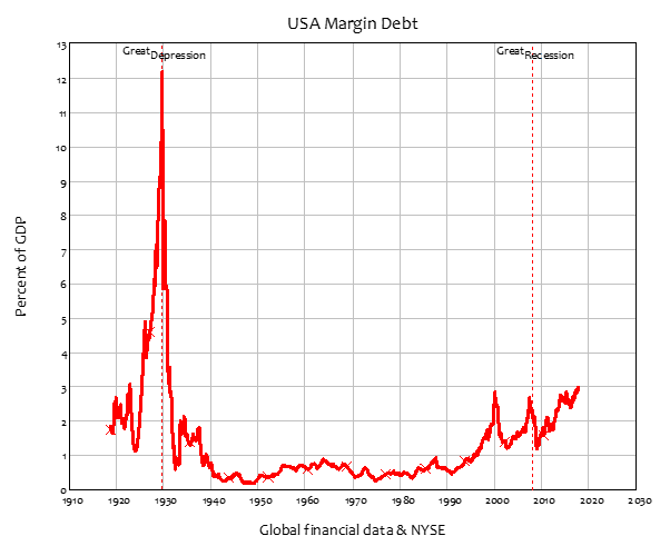
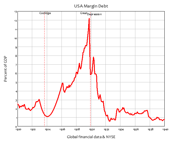
This will mainly be a personal reflection on 2020, but I can’t not post the following chart, showing the level of margin debt and the stock market valuation over the last century. When the Spanish Flu ended, the stock market was at almost its lowest level in history (it hit that level just six months later) and margin debt was comparable to today’s levels, which are six times the post-WWII median of about 0.5% of GDP, but exploded during the 1920s to 13% of GDP (after adjusting pre-WWII data slightly to match post-WWII records).

Especially when combined with the historically high levels of private debt, I simply can’t see the 2020s being anything like the 1920s.

Instead, I think it will be the decade where our foolishness in trusting economists on climate change comes back to bite the economy big-time.

For me, 2020 has been a year of enormous change, all driven by Covid-19. I began the year in Amsterdam, where I had bought a flat with my partner Nisa. I’ve ended it in Bangkok, where we fled in March to escape the Netherlands, which has been as much of a shit-show on Covid-19 as the UK or Sweden—and we formalized our relationship by getting married yesterday.

We’ll now look to buy a place here, for both personal and climate-change related reasons. One reason I bought in Amsterdam was that, on some metrics, it was better placed than any other country in Europe to cope well with climate change. The Dutch are the best in the world at managing water, both in terms of keeping it out with dykes, and in managing it in agriculture; and as by far the world’s leading exporter of food in per capita output terms, they were likely to cope better with the climate-change-driven breakdown of agriculture.

Then they made a complete fist of Covid-19, I expect by falling for the same “herd immunity” nonsense as did Sweden, though not as explicitly. This country of 17 million has as bad a record on Covid-19 as the UK.

I was lucky to have the option of moving to Thailand, given Nisa’s nationality: though she has lived in The Netherlands for over 25 years, she is still a Thai citizen, and moving here was straightforward for her. I made the move initially thinking that it would slow down how quickly I would get the virus, thus giving more time for a vaccine to be developed. Until the recent huge outbreak in a Burmese-migrant-worker enclave on the outskirts of Bangkok, it looked like I had instead drawn the Ace of Hearts from the pack, by choosing somewhere that had eliminated the virus completely.

Even with the recent outbreak—which also illustrates the weakness, in our “spaceship Earth” world, of treating any subgroup as something we can just exploit without consequences—I think Thailand will succeed in eradicating its second wave, as The Netherlands blunders into its third.

There are family reasons for having a home here as well—we live in the same suburb as Nisa’s eldest son, and several sisters—but for me it’s also another climate change hedge. Though Thailand is likely to suffer from higher heat thanks to global warming, it isn’t projected to suffer from the “35°C wet bulb” crisis that will hit the Indian subcontinent.

It is also a net food exporter, and the food supply chain is a lot shorter, even in Bangkok, than for any Western city—including Amsterdam. So that implies relative safety, if food supplies are challenged—and prices rise dramatically as a result.

Places like the UK, which imports about 30% of its food, are likely to be severely challenged when food exporters are hit by climate change breakdowns of major weather systems.

My main reason for wanting hedges against climate change, apart from the merely selfish motivation, is that it seems I’m the person who is best placed to expose the fraud that has underpinned the sanguine forecasts of the economic impact of climate change made by Neoclassical economists like Nordhaus. I want to pursue that all the way from academic articles like “The appallingly bad neoclassical economics of climate change” to being an expert witness if, as I hope, they are eventually prosecuted under the developing laws against ecocide.

Looking forward(?) to 2021, I’ll be developing more research to support that critique of Nordhaus and friends, as well as working on monetary policies to address climate change. I have been invited to write a review paper on economic analysis of climate change Proceedings of the Royal Society A, which I’ll start as soon as I finish the first draft of The New Economics: A Manifesto for Polity Press.

I had hoped to finish that book before the end of the year—that is, in less than two days’ time! I’m close, but I won’t make it. However, I think I’ll have it done by the end of the first week of January, and I’ll post that first draft here (for patrons only).

Next cab off the rank—probably simultaneously with Royal Society paper—will be a policy paper on carbon rationing. Having read the drivel on carbon pricing by economists like Nordhaus, I’m convinced that carbon pricing is far too little, far too late, and rationing of carbon (with tradeable Universal Carbon Credits) is the only feasible monetary means to slow down climate change.

I’m also about to apply for another grant from Friends Provident Foundation to continue the development of Minsky. It has come a long way already thanks to their £200,000 grant, and we have a great development team now, with Russell Standish still the chief programmer, but ably supported by Wynand Dednam, whom we’ve been able to employ fulltime thanks to the grant.

There’s a lot more to do though: we have only just started adding new tabs as part of the interface, the plots need a lot of work, we want to be able to import models from other system dynamics programs (to encourage more use of Minsky, which is one of the very few Open Source system dynamics programs). With the grant, we’ve taken Minsky from a program that didn’t support basic editing operations like copy, cut and paste to an up-to-date GUI. Now we need to round out its system dynamics features and make it a first-class presentation tool.

There’s a ton more work in the pipeline—far too much work, and I’m always playing catch-up with my commitments. One day I hope to have a fully-funded research team working with me, but for now I’m very grateful to my Patrons for the support you give me that enables me to do this work full-time. I just wish there wasn’t so much of it!

Keep safe everyone. Vaccines have started to roll out, but there are many months to go before they will enable us to put Covid-19 in the same category as smallpox or polio. You’ll need as much of your good health as you can hang on to to cope with what I think the 2020s have in store for us.

Discussing a Modern Debt Jubilee on Macro’n’Cheese

I discuss a Modern Debt Jubilee On Macro’n’Cheese today, and this is a quick explanation of how it could be done.

Jubilees were common in antiquity. The Lord’s Prayer did not originally say “And forgive us our sins, as we have forgiven those who sin against us”, but “And forgive us our debts, as we also have forgiven our debtors”. But an old-fashioned Jubilee would reward those who gambled with borrowed money, and thus effectively penalise those who did not. It would also effectively bankrupt the banks, since their assets—our debts—would fall, while their liabilities—our deposits—would remain constant.

A Modern Debt Jubilee gets around both problems by:

  • Giving everyone, whether they borrowed or not, exactly the same amount of money; and
  • Replacing risky private debt as an income earning asset for banks with riskless Jubilee Bonds.

The basic mechanics in a Modern Debt Jubilee are:

  • Every adult gets an identical sum of money;
    • Those in debt must pay their debt down by that amount;
    • Those that are not in debt—or have less debt than the Jubilee amount—must buy newly-issued shares directly from corporations;
    • Corporations must use the revenue from share sales to pay down corporate debt;
  • Jubilee Bonds are sold by Treasury to banks; and
    • Interest payments on Jubilee Bonds (partly) compensate for the fall in interest payments on household and corporate debt.

Figure 1: The basic mechanics of a Modern Debt Jubilee

The end-result of a Modern Debt Jubilee is:

  • Debtors are not unfairly advantaged over savers (debtors have less debt, while savers get new debt-free assets);
  • Private debt, both household and corporate, falls, while equity (share ownership) rises;
  • The amount of money does not change a great deal (it changes only by the interest on Jubilee Bonds); and
  • Banks remain solvent, because their assets rise as much as their liabilities, and they gain equity from the interest on Jubilee Bonds.

As with a government deficit, the government doesn’t need to borrow the money given to debtors and savers: the Jubilee creates the money, in the same manner that a deficit creates money. It also creates additional Reserves, on the Asset side of the Banking Sector’s ledger. If the Treasury issues “Jubilee Bonds”, then rather than those bonds involving borrowing money from the private sector, they are an asset swap that lets the banks swap non-income-earning reserves for income-earning bonds.

I’ll go into more detail on the hows, whys and wherefores of a Modern Debt Jubilee in a later post.

Money matters

Most people who haven’t studied economics expect economists to be experts on money—after all, isn’t that what economics is about? In fact, Neoclassical macroeconomics ignores banks, and private debt, and money. Neoclassical economists justified this omission, at least before the 2007 Global Financial Crisis, with the assertion that banks—and their products, debt and money—were largely irrelevant to macroeconomics.

Ex-Federal Reserve Chairman Ben Bernanke put it this way, when he dismissed Irving Fisher’s argument that the Great Depression was caused by a process that Fisher termed “debt-deflation”:

Fisher envisioned a dynamic process in which falling asset and commodity prices created pressure on nominal debtors, forcing them into distress sales of assets, which in turn led to further price declines and financial difficulties… Fisher’s idea was less influential in academic circles, though, because of the counterargument that debt-deflation represented no more than a redistribution from one group (debtors) to another (creditors). Absent implausibly large differences in marginal spending propensities among the groups, it was suggested, pure redistributions should have no significant macroeconomic effects. (Bernanke 2000, p. 24. Emphasis added)

By “pure redistribution”, what Bernanke meant is that, in the Neoclassical model of banking, lending and the repayment of debt transfer money from one group to another—from saver to borrower in the case of lending, and from borrower to saver in the case of repayment—but no new money is created. Unless there is a substantial difference in the rate at which savers and borrowers spend, this model predicts that the macroeconomic impact of a substantial fall in the level of debt—a “debt-deflation”—will be slight.

“Nobel Prize” winner (Offer and Söderberg 2016, Mirowski 2020) Paul Krugman elaborated on this argument in his New York Times column, where he has regularly explained and promoted the “Loanable Funds” model of banking (Krugman 2009, Krugman 2011, Krugman 2011, Krugman 2013, Krugman 2015, Krugman 2015). In this model, banks are intermediaries between “more patient people” who want a return on their savings, and “less patient people” who want to spend more than their incomes at some point in time:

Think of it this way: when debt is rising, it’s not the economy as a whole borrowing more money. It is, rather, a case of less patient people—people who for whatever reason want to spend sooner rather than later—borrowing from more patient people. (Krugman 2012, p. 147)

In this model, lending simply shuffles existing money from one set of people to another: banks take in deposits from some customers, and lend them out as loans to other customers. There is also no relationship between the level of private debt and the amount of money in the economy.

If this
description of how banks operate were correct, the amount of money couldn’t change—just its distribution between the bank accounts of the different customers of the banks. So how could money be created then? In Neoclassical economics, money creation is primarily the province of the government, via what is known as “Fractional Reserve Banking”, or the “Money Multiplier”. A bank, it is asserted, takes in deposits from savers, and then lends out a large fraction of these to borrowers. This lending creates money in an iterative process involving many banks. The amount created is largely determined by the government via its Central Bank, but actions by banks and the non-bank public can only reduce the amount of money created, not increase it. Gregory Mankiw explains it in this way his textbook Macroeconomics:

If the Federal Reserve adds a dollar to the economy and that dollar is held as currency, the money supply increases by exactly one dollar. But as we have seen, if that dollar is deposited in a bank, and banks hold only a fraction of their deposits in reserve, the money supply increases by more than one dollar. As a result, to understand what determines the money supply under fractional–reserve banking, we need to take account of the interactions among (1) the Fed’s decision about how many dollars to create, (2) banks’ decisions about whether to hold deposits as reserves or to lend them out, and (3) households’ decisions about whether to hold their money in the form of currency or demand deposits. (Mankiw 2016, pp. 93-94)

There are three factors that determine the money supply in this model: the “monetary base”, which “is directly controlled by the Federal Reserve”; the fraction of any bank deposits that banks hold on to, which “is determined by the business policies of banks and the laws regulating banks”, and the amount of money the public hold in cash versus the amount they deposit in banks.

The only point in this model at which banks have an active role is their capacity to hold a higher fraction of deposits as reserves than they are required to do by law, and the only impact this can have is to reduce the amount of money created. Bank customers can also reduce the amount of money created by keeping more of their money as cash. The Central Bank therefore has the dominant role in determining the money supply, according to Neoclassical economics. For this reason, in his Essays on the Great Depression, Bernanke blamed the calamity of the Great Depression on the Federal Reserve itself:

our analysis provides the clearest indictment of the Federal Reserve and U.S. monetary policy. Between mid-1928 and the financial crises that began in the spring of 1931, the Fed not only refused to monetize the substantial gold inflows to the United States but actually managed to convert positive reserve inflows into negative growth in the M1 money stock. Thus Fed policy was actively destabilizing in the pre-1931 period… our methods attribute a substantial portion of the worldwide deflation prior to 1931 to these policy decisions by the Federal Reserve. (Bernanke 2000, p. 111)

In contrast, Post Keynesian economists followed Irving Fisher (Fisher 1932, Fisher 1933) and blamed the Great Depression on the disequilibrium dynamics of private debt. Hyman Minsky combined Fisher’s ideas with Keynes’s to develop what he christened the “Financial Instability Hypothesis” (Minsky 1963, Minsky 1975, Minsky 1977, Minsky 1978). Private debt, which Neoclassical economists ignore, was an essential component of Minsky’s analysis of the instability of capitalism. He put it this way:

The natural starting place for analyzing the relation between debt and income is to take an economy with a cyclical past that is now doing well… As the period over which the economy does well lengthens, two things become evident in board rooms. Existing debts are easily validated and units that were heavily in debt prospered; it paid to lever… As a result, over a period in which the economy does well, views about acceptable debt structure change… As this continues the economy is transformed into a boom economy.

Stable growth is inconsistent with the manner in which investment is determined in an economy in which debt-financed ownership of capital assets exists, and the extent to which such debt financing can be carried is market determined. It follows that the fundamental instability of a capitalist economy is upward. The tendency to transform doing well into a speculative investment boom is the basic instability in a capitalist economy. (Minsky 1982, p. 66. Emphasis added)

For rising debt to cause rising economic activity, there must be some mechanism by which rising debt boosts aggregate demand—in contrast to the Neoclassical argument that changes in the level of debt were “pure redistributions” with “no significant macroeconomic effects” (Bernanke 2000, p. 24 ). The Neoclassical “Loanable Funds” and “Fractional-Reserve-Banking—Money Multiplier” models must therefore be wrong: bank lending must somehow create money, and this must also increase aggregate demand.

Post Keynesian economists—and some policy economists in Central Banks as well (Holmes 1969)—have argued for many decades that these Neoclassical models are false, and that banks create money when they lend (Fisher 1933, Schumpeter 1934, Minsky 1963, Moore 1979, Moore 1988, Graziani 1989, Minsky 1990, Minsky and Vaughan 1990, Keen 1995, Moore 1997, Moore 2001, Fontana and Realfonzo 2005, Fullwiler 2013, Werner 2014, Werner 2014), but their protestations were ignored by Neoclassicals. However in 2014, no less an institution than the Bank of England sided with the Post Keynesians (McLeay, Radia et al. 2014, McLeay, Radia et al. 2014, Kumhof and Jakab 2015, Kumhof, Rancière et al. 2015), and stated emphatically that the Neoclassical models of banking—”Loanable Funds”, “Fractional Reserve Banking” and “The Money Multiplier”—were false:

The reality of how money is created today differs from the description found in some economics textbooks:

  • Rather than banks receiving deposits when households save and then lending them out, bank lending creates deposits.
  • In normal times, the central bank does not fix the amount of money in circulation, nor is central bank money ‘multiplied up’ into more loans and deposits. (McLeay, Radia et al. 2014, p. 1. Emphasis added)

The Bundesbank made a similar pronouncement in 2017:

It suffices to look at the creation of (book) money as a set of straightforward accounting entries to grasp that money and credit are created as the result of complex interactions between banks, non- banks and the central bank. And a bank’s ability to grant loans and create money has nothing to do with whether it already has excess reserves or deposits at its disposal. (Deutsche Bundesbank 2017, p. 13. Emphasis added)

Neoclassical economists could not completely ignore these flat-out contradictions of their models of banking by establishment bodies like Central Banks, but rather than accepting the critique and abandoning their models, their reaction was defensive. For example, Krugman argued that the Bank of England’s paper was nothing new—and therefore it did not challenge the relevance of the Loanable Funds model, even though the model itself was technically wrong:

OK, color me puzzled. I’ve seen a number of people touting this Bank of England paper (pdf) on how banks create money as offering some kind of radical new way of looking at the economy. And it is a good piece. But it doesn’t seem, in any important way, to be at odds with what Tobin wrote 50 years ago … Don’t let monetary realism slide into monetary mysticism! (Krugman 2014. Emphasis added)

Since then, Neoclassical textbooks have continued to teach the Loanable Funds and Fractional Reserve Banking models of banking (Mankiw 2016, pp. 71-76, 89-100), as if there’s nothing wrong in teaching factually incorrect models—as if the change from a model in which banks do not create money, to one in which they do, makes no difference to macroeconomics.

However, the fact that banks create money when they lend has an enormous impact on macroeconomics, and models which pretend that banks don’t create money are utterly inaccurate models of capitalism. This can be seen simply by contrasting Bernanke’s dismissal of Fisher’s debt-deflation explanation for the Great Depression with the data. Bernanke asserted that the change in debt (which he called a “pure redistribution”, following the Loanable Funds model of banking) should have “no significant macroeconomic effects” (Bernanke 2000, p. 24). That can be framed as the statistical hypothesis that the correlation coefficients between the change in private debt and important macroeconomic variables should be not significantly different from zero.

In fact, the correlation between credit (the annual change in private debt, measured in percent of GDP) and employment between 1920 and 1940 was 0.81. Between 1990 and 2020, it was as 0.82 (see Figure 1).

Figure 1: The correlation between credit and employment across 1990-2020 was 0.82
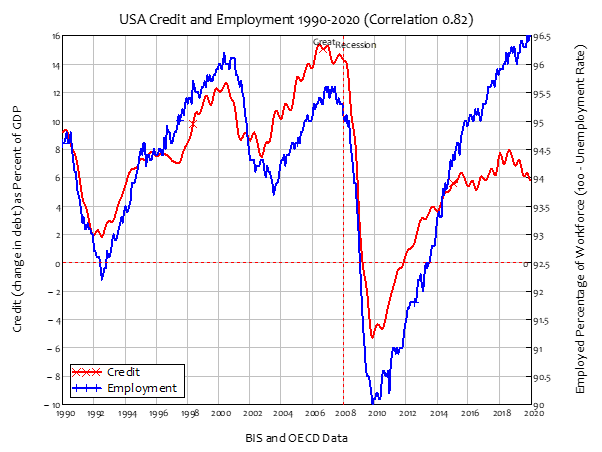
There is therefore a striking anomaly between Neoclassical economic theory and the real world. Let’s investigate this anomaly—and start constructing a new, monetary approach to economics—using one of the new computer software tools I alluded to earlier: the Open Source (that is, free) “system dynamics” program Minsky.

  1. Modelling Credit Money in Minsky

Minsky was built to model money, which raises the vexed question “Well, what is money?”. The question is vexed because, especially today, people hold vehement views about what money should be—rather than what it currently is. Some argue that gold is money (Sennholz 1975); others assert that crypto-currencies should be money (Chambers 2019). However, in practical terms, gold and cryptocurrencies primarily fulfil only the last of the three accepted characteristics of money: a unit of account, a means of payment, and a store of value. The first two characteristics, which are essential to commerce in a market economy, are today fulfilled predominantly by national currencies.

Secondly, the vast majority of transactions today involve, not transfers of physical notes and coins, but electronic transfers between bank accounts, in return for goods. This is an exchange of records in a computer database, in return for a commodity or a service. The Post Keynesian monetary theorist Augusto Graziani pointed out that this meant that “any monetary payment must therefore be a triangular transaction, involving at least three agents, the payer, the payee, and the bank” (Graziani 1989, p. 3).

Banks themselves developed out of the double-entry bookkeeping system designed by accountants to keep track of financial commitments (Gleeson-White 2011): all transactions are recorded twice, once from the source account and once in the destination account. Accounts are classified as Assets, Liabilities, or Equity, following the rule that Assets minus Liabilities equals Equity. Minsky employs these accounting rules to build macroeconomic models based on monetary transactions, using double-entry bookkeeping tables we call “Godley Tables”.

This method of modelling money is both remarkably simple and remarkably powerful. It can easily demonstrate the key differences between Loanable Funds and a realistic model of what banks actually do, which I call “Bank Originated Money and Debt” (BOMD)—see Figure 2.

Figure 2: Loanable Funds versus Bank Originated Money and Debt

The first table in Figure 2 shows the basics of the Loanable Funds model of banking, in which banks do not create debt themselves, but facilitate lending from one group of non-Bank entities (“Savers”) to another (“Borrowers”). The key features of this false, Neoclassical model of banking are:

  • Money is the sum of the amounts in the Liability and Equity accounts of the banking sector;
  • Banks don’t lend money. Instead, they facilitate loans between some of their customers (“Savers”) and others (“Borrowers”);
  • The lending and repayment action occurs on the Liabilities side of the banking sector’s ledger—nothing happens on the Asset side;
  • Because Loans are neither an Asset nor a Liability of the Banks, Loans don’t appear on the Banking Sector’s ledger;
  • Reserves are needed to back the deposits made by savers, borrowers, and the banking sector itself;
  • Interest income on loans accrues to Savers rather than to the Banks;
  • Banks earn income not from interest on loans, but from charging “intermediation fees” to borrowers or savers; and
  • Finally, and most importantly for the significance of banking in macroeconomics, money is neither created by lending, nor destroyed by repayment. Instead the existing stock of money in this model is shuffled between the bank accounts of Savers and Borrowers.

The second table in Figure 2 shows the basics of actual lending, with the differences between real-world lending and the Loanable Funds model highlighted in italics:

  • Money is the sum of the amounts in the Liability and Equity accounts of the banking sector;
  • Banks do lend money;
  • The lending and repayment action occurs on both the Assets and the Liabilities side of the banking sector’s ledger. Lending increases Loans, which are an Asset of the banking sector, and it also increases the deposit accounts of Borrowers—which are Liabilities of the banking sector. Repayment reduces the banking sector’s Assets (Loans) and Liabilities (Deposit accounts);
  • Loans are Assets of the banking sector (Reserves don’t appear in this simplified model, because they’re not involved in lending—a topic I’ll return to below);
  • Interest income accrues to the banking sector: one of its Liabilities (the deposit accounts of Borrowers) falls and its Equity rises; and
  • Finally, and most importantly for the significance of banking in macroeconomics, money is created by lending and destroyed by repayment.

The only thing these two models agree upon is the definition of money. It would be astounding if they didn’t have different predictions for the impact of bank lending on the economy.

Figure 3: A quick primer on Minsky

Using Minsky, it’s easy to show how profoundly different these predictions are. Figure 4 shows a model of Loanable Funds in which:

  • Capitalists lend to Firms;
  • Firms hire Workers, pay dividends and interest to Capitalists, and intermediation fees to the Banks; and
  • Capitalists, Workers and Bankers buy the output of the Firm sector.

The rates of lending and repayment have been varied during the simulation, so that credit—the difference between new loans and the repayment of old loans—is positive for a while, then negative, then positive again, and finally neutral. This results in large changes in debt, from 50% of GDP to over 150%, and then back again. The changes in the level of debt have some impact on GDP and incomes, but they move in the opposite direction: GDP falls with rising private debt, and rises with falling private debt. But there is no impact of changing levels of private debt upon the total money supply: this remains fixed at $200 billion throughout the simulation.

Figure 4: A Loanable Funds model in which capitalists lend to firms

This model can be easily converted into the real-world model of “Bank-Originated-Money-and-Debt” (BOMD), simply by showing Loans as an Asset of the Banks, rather than the Capitalists. Interest payments are shifted from Capitalists to Banks as well, and the superfluous Fee to banks is deleted. The result is a dramatically different vision of how a monetary economy works. Most importantly, the rising level of debt causes a rising level of money: as debt rises and falls, so does the money supply. Also, rather than the debt to GDP ratio and GDP moving in opposite directions, they move in the same direction: a rising debt to GDP ratio causes a rising level of income, and falling debt causes falling income.

Figure 5: A Bank Originated Money and Debt model where banks lend to firms

These simulations show that the real world of “Bank Originated Money and Debt” is vastly different to the Neoclassical fantasy model of Loanable Funds. But why is it so? How does credit add to aggregate demand?

  1. The logic of credit’s role in aggregate demand

One of the guiding principles of macroeconomics is that one person’s expenditure is another person’s income. Thus, if you spend $250 a year at your local Pizza shop, the sum of your expenditure on Pizza (minus $250 from your bank account) and the Pizza shop’s income from you (plus $250 into the Pizza shop’s bank account) is zero. This is because what is an expenditure to you (buying the pizza) is an income to the recipient (selling the pizza). Expenditure and income are two perspectives on precisely the same transaction.

The same principle applies at the macroeconomic level: expenditure IS income.

We can use this to construct a table showing expenditure and income for any economy, where the rule is that each row shows expenditure by one entity on all other entities in the economy, and that row must sum to zero. Let’s divide the economy into three sectors—say, Manufacturing, Services, and Households, and use capital letters to indicate spending per year by each sector on the other two: so Manufacturing spends A dollars per year on Services, and $B per year on Households. Table 1 shows this view of the economy—which I have named a Moore Table after the Post Keynesian economist Basil Moore (Moore 1979). Notice that each row sums to zero, that each column can differ from zero, and that the whole table sums to zero.

Table 1: A Moore Table showing expenditure IS income for a 3-sector economy

We can now classify parts of the table as aggregate expenditure and aggregate income. The negative of the sum of the diagonal elements is aggregate expenditure. The sum of the off-diagonal elements is aggregate income. They are necessarily identical.


Table 1 is a monetary economy without lending. We can modify it to show the Neoclassical vision of lending, Loanable Funds, by imagining that one sector (say, Services) lends Credit dollars per year to another sector (say, Households), and then Households use this borrowed money to buy more goods from Manufacturing. However, the lending by Services lending comes at the expense of the Service Sector’s spending on Manufacturing (you can’t spend money you’ve lent to someone else). So Services spends (D-Credit) dollar per year on Manufacturing, whereas Households spend (B+Credit) dollars per year on Manufacturing. Lending from the Services Sector to the Household Sector is neither Expenditure nor Income, so the transfer of money can’t be shown horizontally: it is instead shown as a transfer across the diagonal, reducing the expenditure of the lender (Services) and increasing the spending of the borrower (Households). Households pays Interest dollars per year on its outstanding debt to Services, and since this is both an expenditure and an income, it is shown horizontally.

Table 2: The Moore Table for Loanable Funds

When you add up expenditure and income in this table, Credit cancels out: for every positive entry for Credit in either Aggregate Demand (the negative of the sum of the diagonal cells) or Aggregate Income (the sum of the off-diagonal cells), there’s an offsetting negative entry that cancels it out. The only effect of lending on this model of the economy is that Interest payments turn up as part of both expenditure and income:


Table 3 shows the real-world situation of “Bank Originated Money and Debt”. It’s more complicated than the other tables, because we have to add the Banking Sector to the model, and we have to include the Banking Sector’s Assets—where Credit appears as an increase in the Banking Sector’s loans to the Household Sector—as well as its Liabilities and its Equity. Table 3 explicitly shows all spending as passing through the Liabilities (Deposit accounts) and Equity sides of the banking sector’s accounts. The Household Sector’s expenditure on Manufacturing includes Credit, as in Loanable Funds, but this credit-financed spending does not come at the expense of any other sector’s expenditure: instead, it comes from the creation of new money via the expansion of the Banking Sector’s Liabilities and Assets.


Table 3: The Moore Table for Bank Originated Money and Debt

The key outcome is that Credit does not cancel out, as it does in Loanable Funds: there is a single entry for Credit in Aggregate Expenditure—it finances part of the Household Sector’s purchases from the Manufacturing Sector—and a single entry in Aggregate Income—where it is part of the Manufacturing Sector’s income:


Consequently, in the model shown in Table 3—and in the real world—credit is a substantial source of both Aggregate Demand and Aggregate Income. This is the logical explanation of the difference in behavior between the “Loanable Funds” model shown in Figure 4 and the BOMD model shown in Figure 5. It is also the explanation for the real-world phenomena of debt-deflationary crises like the Great Recession, the Great Depression, and the Panic of 1837. Neoclassical economics, by ignoring banks, debt and money in its macroeconomic models, is ignoring the main factors that drive economic performance, and also cause economic crises.

  1. Negative credit, economic crises, and economic policy

Neoclassical economists appropriated Nassim Taleb’s phrase “The Black Swan” (Taleb 2010) to assert that the Great Recession was impossible to predict, because crises like it are so rare, and because their causes are fundamentally random. Called “exogenous shocks” by Neoclassicals, random events are the only factors that cause Neoclassical models of the economy to deviate from equilibrium. So, “exogenous shocks” must have caused the Great Recession. The Boston College Economics Professor Peter Ireland put it this way:

In terms of its macroeconomics, was the Great Recession of 2007–09 really that different from what came before? The results derived here from estimating and simulating a New Keynesian model provide the answer: partly yes and partly no.

These results suggest that largely, the pattern of exogenous demand and supply disturbances that caused the Great Moderation to end and the Great Recession to begin was quite similar to the patterns generating each of the two previous downturns in 1990–91 and 2001. Compared to those from previous episodes, however, the series of adverse shocks hitting the U.S. economy most recently lasted longer and became more intense, contributing both to the exceptional length and severity of the Great Recession. (Ireland 2011, p. 51).

The policy prescription from this analysis is … to do nothing at all, beyond the Boy Scout motto of “be prepared”. From the perspective of the Neoclassical paradigm, crises like the Great Recession can’t be anticipated, let alone made less likely by economic policy. We can only deal with their consequences after they happen.

This is akin to Aristotle’s theory of comets (which was preserved in Ptolemaic astronomy) that comets were unpredictable, because they were atmospheric phenomena (Aristotle and (translator) 350 BCE [1952], Part 7). The Copernican scientific revolution, which overthrew this worldview, showed that comets were inherently predictable, as they are celestial objects orbiting the Sun.

Similarly, the “unpredictability” of crises like the Great Recession is a product of the Neoclassical paradigm’s false Loanable Funds model of money. The correct Bank Originated Money and Debt model shows that crises are caused by credit turning negative (Vague 2019), and that most recessions are caused by credit declining, but not quite going negative. This causal relationship between credit (which is identical in magnitude to the annual change in private debt) and economic performance endows capitalist economies with a tendency to accumulate higher and higher levels of private debt. This phenomenon is most evident in that most capitalist of economies, the United States of America—see Figure 6.

Figure 6: Private Debt and Credit in the USA since 1834
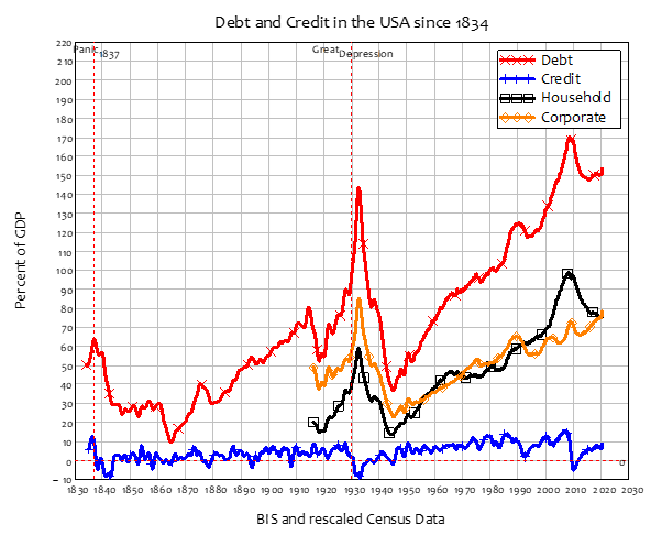
This chart identifies America’s three great economic crises: the Great Recession, the Great Depression, and the “Panic of 1837”. What, you haven’t heard of the “Panic of 1837”? Neither had I, until I produced this chart (Census 1949, Census 1975), but after doing so, I found it was described at the time as “an economic crisis so extreme as to erase all memories of previous financial disorders” (Roberts 2012, p. 24). In each of these crises, credit plunged from a historically high level, turned negative, and remained negative for a substantial period—see Table 4.

Table 4: Magnitude of Credit and duration of negative credit in the USA’s major economic crises

Each crisis turned around only when the decline of credit stopped. But the renewed growth engendered by rising credit came at the expense of a rising private debt to GDP ratio, with this rise terminated either by another crisis, or by wars that drove the private debt ratio down dramatically because of the “War Economy” boost to GDP: nominal GDP growth reached 32% p.a. during the US Civil War in (1861-65), 29% during WWI (1914-1918), and 29% again during WWII (1939-45), far exceeding the maximum growth rate of credit during those periods (0.2% of GDP p.a., 8.6% and 4.5% respectively).

This is no way to run an economy, but it is what we are stuck with while economic policy is dominated by a theory of economics that ignores banks, private debt, money, and credit. However, with a new, monetary paradigm, several things become evident: we should stop the level of private debt from getting too high, and credit-based demand should not be allowed to become too large a component of aggregate demand. But how could we do that?

It’s time to take a monetary look at the other type of debt: government debt.

  1. Modelling Fiat Money in Minsky

Minsky can model government money creation—fiat money—just as easily as it can credit money. Figure 7 shows the basic monetary operations of a government involve spending on the public (either via purchases of goods or direct income support), taxing the public, selling bonds to the financial sector to cover any gap between spending and taxation, paying interest on those bonds, the Central Bank buying some of those bonds off financial entities in “Open Market Operations”, and Banks selling Treasury Bonds to the non-bank private sector.

Figure 7: The fundamental monetary operations of the government

Though a complete picture requires looking at the Central Bank and Treasury balance sheets as well (see Figure 8), several facts about government financing can be deduced from it that are the opposite of conventional beliefs—conventional beliefs which originate with Neoclassical economists, and are promulgated in their textbooks, such as Mankiw’s Macroeconomics (Mankiw 2016).

Firstly, Neoclassicals allege that the government has to borrow from the public to finance any excess of government spending over taxation:

When a government spends more than it collects in taxes, it has a budget deficit, which it finances by borrowing from the private sector or from foreign governments. The accumulation of past borrowing is the government debt. (Mankiw 2016, p. 555. Emphasis added)

Secondly, they claim that this debt burdens future generations:

“government borrowing reduces national saving and crowds out capital accumulation… Many economists have criticized this increase in government debt as imposing an unjustifiable burden on future generations” (Mankiw 2016, pp. 556-57)

Figure 7 shows that the first conventional (Neoclassical) belief is the exact opposite of the truth. Firstly, when government spending exceeds taxation (when Spend is greater than Tax in Figure 7) then the amount of money in the private sector increases by the same amount: government spending increases the Deposits of the non-bank, non-government sector of the economy. This means that the Banking Sector’s liabilities to the Non-Bank Private Sector rise, and this is matched by an identical increase in the Banking Sector’s assets of Reserves. Since both the Assets and the Liabilities of the Banking Sector have risen, and money is the sum of the Liabilities and Equity of the Banking Sector, then the deficit has created money (Kelton 2020). The government doesn’t need to borrow what it has already created.

But what about the sale of Treasury Bonds to the Banking Sector? Is that borrowing? Technically yes, because Treasury Bonds are a debt of the government to the holder of those bonds. But where does the Banking Sector get the money it uses to buy these bonds? The real-world process is more complicated, but fundamentally, as well as creating additional money (when Spend is greater than Tax in Figure 7) the deficit creates an identical amount of Reserves. Reserves are an Asset of the Banking Sector that normally earns no interest. So, when the government then offers to sell Treasury Bonds equal to the size of the deficit, it is presenting the Banking Sector with an offer to convert non-income-earning Reserves into income-earning Treasury Bonds. This is why every sale of Treasury Bonds in history has been not merely successful, but oversubscribed: an auction of Treasury Bonds is an offer to convert a non-income-earning gift (the additional Reserves created by the deficit) into an income-earning one (Treasury Bonds). Of course, the Banking Sector takes advantage of that offer.

What would happen if the Treasury didn’t sell the bonds—so that all the bond-related flows in Figure 7 would not exist? Money creation would still occur, because, in that case, the only entries in the Liabilities & Equity side of the Banking Sector’s accounts would be Spend minus Tax: the deficit itself creates money, regardless of whether or not bonds are sold to cover the deficit. The consequences of not selling bonds therefore lies elsewhere in the financial system.

The Treasury’s balance sheet in Figure 8 (the 3rd table in the Figure) shows what these are. The first column is the Treasury’s “deposit account” at the Central Bank. Without the bond sales, the only guaranteed flows into and out of that account are Tax minus Spend—the same terms as for the creation of money, but with the opposite sign. Therefore, the impact of the government not selling bonds equal to the deficit each year would be that, with sustained deficits over time, the Treasury’s deposit account at the Central Bank would go negative—it would turn into an overdraft account.

For a private entity, an overdraft at a private bank means a much higher interest rate than on a standard loan on the negative balance in its deposit account, limits on how high the overdraft can be, other possibly punitive measures, and the prospect, if the overdraft gets too large, of bankruptcy. But for the Treasury, there are no such consequences, since the Treasury is the effective owner of the Central Bank. In some countries, the Treasury is required by law to pay interest to the Central Bank on any loans, including overdrafts, but in all countries, the profits of the Central Bank are remitted to the Treasury—so in effect the Treasury pays zero interest on its “debt” to the Central Bank. There are effectively no consequences for the Treasury from having an overdraft at the Central Bank.

All bond sales do is enable the Treasury to avoid an overdraft, by keeping its Central Bank account positive (or at least non-negative). Most governments have passed laws requiring its Treasury to not be in overdraft to its Central Bank—though these laws were waived by some countries during the Covid-19 crisis. New laws, based on a realistic appreciation of the role of government money creation in a well-functioning economy, could enable the Treasury to always run an overdraft—or let it run up a debt to the Central Bank—obviating the need to sell bonds at all.

What about the interest on Treasury Bonds? That can be paid by the Treasury borrowing from the Central Bank—(the term LendCB in Figure 7)—and thus adding to a loan on which it effectively pays zero interest. This is a case of the government being in debt to itself, and only for the interest it pays on the bonds it has sold.

The interest payments themselves are another way in which the government creates fiat money in the non-Government sector, this time by adding to the equity of the Banking Sector (or whoever the Banking Sector has sold bonds to). Banks would be the first to complain if the government decided to stop issuing bonds, and took away an easy source of bank profits.

Figure 8: The same operations including the perspective of the Central Bank, Treasury and Non-Bank Private Sector

The Central Bank also does not “monetize” the government deficit when it buys Treasury Bonds off the Banking Sector. This common expression is simply wrong, because the deficit is already “monetized”: to labour the point illustrated by the first two rows of Figure 7, the deficit itself creates money when it increases the Liabilities of the Banking Sector (Deposits) and the Assets (Reserves). Central Bank purchases of Treasury Bonds from the Banking Sector undo the effect of the Treasury selling those bonds to the Banking Sector in the first place: they replace income-earning assets in the Banking Sector’s portfolio (Treasury Bonds) with non-income-earning ones (Reserves). The Banks wouldn’t do the trade without making a profit, but the end-result is they end up with a lower income stream, since they no longer get the interest Treasury pays on those bonds. Far from “monetizing” the deficit, Central Bank bond purchases reduce the amount of money created by the government, since they reduce the amount of interest paid to the Banking Sector.

The only use of Bonds that affects the money supply is the sales of bonds by the Banks to the non-Bank private sector (shown as the second last row in Figure 7), and this destroys money, rather than either creating it, or providing money to the government for it to spend. When Banks sell Treasury Bonds to non-Banks, the deposits of the non-Banks fall, as do the Bank’s own assets of Bonds. This destroys money. Rather than such sales being a source of revenue for the government, they are a source of trading profits for the Banks, and a way to reduce the spending power of the public.

This realistic perspective on government spending upends the conventional wisdom of Neoclassical economics. The government does not “borrow from the private sector” when it runs a deficit. Instead, a deficit creates “debt free” money for the private sector. The deficit increases private savings, rather than reducing them, as Mankiw alleges: the ledger for the Non-Bank Private Sector in Figure 8 shows that the equity of the public (the column PublicEquity in Figure 8) is increased by a deficit (when Spend exceeds Tax) and reduced by a surplus. Deficit thus make it less necessary for households and firms to borrow money from the private banks, while also providing the private banks with a guaranteed source of income, which makes them less likely to want to sell speculative financial assets to the non-bank private sector.

Therefore, far from government deficits “burdening future generations”, they enrich current generations. Any impact on future generations depends on the economic and political consequences of the spending which generates the deficit, and they can be substantially beneficial to the private sector, rather than deleterious. Consider, for example, the enormous deficits of up to 25% of GDP, and the resulting trebling of government debt (from 38% to 109% of GDP) caused by government spending during World War II (see Figure 9). Without that deficit—which, as we have seen above, was funded by fiat money creation, not by borrowing from the public or the banks—and corresponding ones for its allies (the UK’s deficit hit 44% of GDP in 1941), the Axis powers would have won WWII.

Figure 9: US Government debt and deficits over the past 120 years
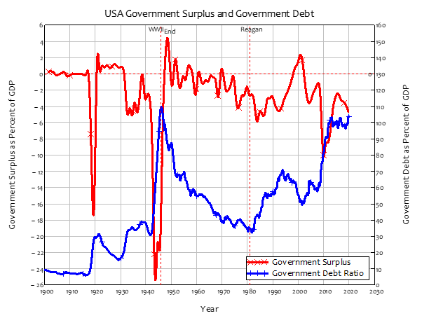
Deficits of that scale rapidly increased the government debt to GDP ratio, to 110% of GDP—the highest in America’s history. According to Mankiw and almost all Neoclassical economists, this should have placed an enormous burden on the “future generation” that followed the wartime one. So how did this unfortunate cohort fare?

I speak, of course, of the Baby Boomers. Born between 1946 and 1964, they were probably the most privileged generation in human history. Far from suffering pain from having to repay the enormous government debts accumulated during WWII, their time in the sun coincided with the “Golden Age of Capitalism” (Marglin and Schor 1992) between 1950 and 1973. They experienced high growth, low unemployment, low inflation, and—in an apparent paradox—a falling government debt to GDP ratio, while the budget was normally in deficit (see Table 5). If that’s being burdened, then please, bring it on.


Table 5: Economic performance of major periods in post-WWII USA

  1. An integrated view of deficits and credit

One striking feature of Figure 9 is the rarity of government surpluses, despite the never-ending political rhetoric about achieving them. The only period of sustained surpluses was the 1920s, when the government maintained a surplus of roughly 1% of GDP each year. The “Roaring Twenties”, as the decade became known, was a time of great economic prosperity, and in his 1928 State of the Union Address, then President Calvin Coolidge attributed this success to the government surplus:

No Congress of the United States ever assembled, on surveying the state of the Union, has met with a more pleasing prospect than that which appears at the present time…

a surplus has been produced. One-third of the national debt has been paid… the national income has increased nearly 50 per cent…. That is constructive economy in the highest degree. It is the corner stone of prosperity. It should not fail to be continued. (Coolidge 1928)

In fact, the surplus was depressing the economy, by taking the equivalent of just under 1% of GDP out of private bank accounts every year. The public responded by borrowing on average 5% of GDP every year, and using this to gamble on financial assets—initially housing in a forgotten but significant housing bubble (Vague 2019), and then in the stock market—in an orgy of debt-fueled speculation. As Coolidge lauded himself for causing government debt to fall from 30% to 15% of GDP, private debt rose from 55% to 100% of GDP—so that for every one dollar of (for the private sector) debt-free fiat money Coolidge removed from the economy, the private sector pumped $3 of debt-based money back in.

We can avoid Coolidge’s mistake of attributing all of the economy’s performance during the 1920s to the government surplus by building a simple Minsky model with both a government, and a banking sector that lends to the non-bank public: see Figure 10. I did three simulations: one with the Coolidge-era settings of a 1% of GDP government surplus and credit at 5% of GDP; one with a balanced budget and credit at 5%; and one with a 1% of GDP surplus and no credit.

Figure 10: An integrated view of government deficits and private sector credit

The first setting led to the “pleasing prospect” of which Coolidge waxed lyrical. Over a ten-year simulation, GDP rose from $560 billion to $1660, and the government debt ratio fell from 30% of GDP to 2%. But the model economy did better still with a balanced budget. GDP hit $2,000 billion, and the government debt ratio still fell to 7.5%. More tellingly, with the boost from credit removed—with a 1% of GDP surplus and zero credit, and therefore no growth in private debt—the economy slumped. GDP peaked at $750 billion after 3 years and fell thereafter, reaching $700 billion after ten years on a sustained downward trajectory, while the government debt ratio fell less (to 11% of GDP) because GDP was falling as well as government debt.

This model actually flatters Coolidge and the 1920s, because borrowing in it boosts GDP via investment by firms and consumption by workers and banks. But during the 1920s, much of the borrowing went into speculation. The most spectacular instance of this was the unprecedented, and unsurpassed, level of margin debt, which rose from 1% of GDP in the early 20s to 13% in October 1929—see Figure 11. This is why the Twenties roared—and largely also why the Thirties wailed.

Figure 11: Margin debt since 1918
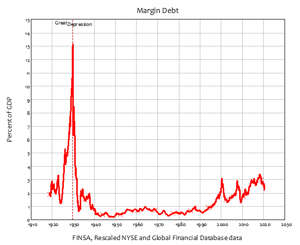
Margin debt enabled a speculator to put down a deposit of $1,000 with a stockbroker and borrow $9,000, to buy $10,000 worth of shares with a $10,000 “margin account”. The borrower paid interest on the loan of course, but the leverage meant that, if markets rose 10%, then before expenses, the speculator doubled his money: $10,000 worth of shares became $11,000, doubling the speculator’s net worth from $1,000 to $2,000. There was a catch: if the market fell 10%, then the speculator had to top up the account to keep it at $10,000. This would wipe the speculator’s equity out—from $1,000 to zero (before expenses). If the speculator couldn’t comply with his ready cash, then the stockbroker was entitled by the margin contract to liquidate any of the speculator’s assets: it was an unlimited liability. But most speculators were confident that this would never happen, and over the course of the decade, they were right: while the margin debt to GDP ratio increased 5.5 times between the stock market’s all-time low point in 1921 and October 1929, the stock market itself rose sixfold.

Few were more confident than Professor Irving Fisher, who was his day’s Paul Krugman: a famous mainstream economist (and also inventor) who also wrote a column for the New York Times. He had levered the profits from inventions into the stock market, and became its most prominent cheerleader. On October 16th 1929, Fisher was quoted in the Times as saying at a conference that “Stock prices have reached what looks like a permanently high plateau.” He continued:

I do not feel that there will soon, if ever, be a fifty or sixty point break below present levels, such as Mr. Babson has predicted. I expect to see the stock market a good deal higher than it is today within a few months. ( “Fisher sees stocks permanently high“) (Fisher 1929, October 16th, p. 8. Emphasis added)

Just two weeks later, the Dow Jones Industrial Average plunged over 60 points in two days, losing more than 20% of its value. Margin calls wiped out levered speculators like Fisher immediately, and ushered in The Great Depression, which itself did much to cause the rise of fascism and the Second World War.

As awful as those crises were, they had one strong positive economic side-effect, from which the next generation—the Baby Boomers—benefited handsomely. The combination of massive government spending and constrained private sector consumption during WWII enabled the deleveraging that commenced in 1933 to continue. By the end of WWII, private debt had fallen to 40% of GDP from its debt-deflation-driven peak of 144% in 1932 (see Figure 6). This low level of private debt, along with the substantial level of fiat-based money created during WWII, low interest rates, and regular government deficits, meant that the financial burden on the private sector in the 1950s and 1960s was trivial. It was as if the slate had been wiped clean by a classical Jubilee.

Not realizing any of this, and certainly not understanding the incredible reluctance of their parents and grandparents to go into debt, the Baby Boomers restarted the borrowing bubble, culminating in the telecommunications, dotcom, and finally Subprime bubbles, which drove private debt to its highest level in American history (and in most of the rest of the developed world).

Contrast that to today, where private debt fell by only 20% from its Great Recession peak of 170% of GDP. It still sits above the previous peak that it was driven to by deflation in 1932. We need to reduce private debt back to its levels during that Golden Age—but we should find a better way of doing so than another World War.

  1. A Modern Debt Jubilee

The monetary perspective developed in the previous sections shows that the real-world roles of private and public debt, and of credit and government deficits, are the exact opposite of what the Neoclassical conventional wisdom asserts. Private debt, not government debt, is the primary cause of economic crises. Credit, and not government deficits, is dangerous when it is large relative to GDP. Rising private debt, not rising government debt, is the main indicator of an approaching crisis. Private debt, not government debt, can depress economic activity because it is too high. These insights indicate that the levels of private debt and credit are economic indicators of at least as much importance as the customary ones of the unemployment rate and the inflation rate. They should be monitored as closely, and economic policy should aim to keep them both relatively low.

But that leaves the issue of what to do after Neoclassical economics, by not merely ignoring private debt, but by actively arguing in favor of debt-financing of business (Modigliani and Merton 1958), has helped drive private debt to at least three times its Golden Age level. If capitalism is ever to have another Golden Age—and one will be needed to address the challenges of Climate Change—then we need to reduce the private debt to GDP ratio by at least as much as it was reduced during the 1930s and 1940s. This could be done in exactly the same way that the government runs a deficit today, in a way that does not advantage those who gambled with borrowed money over those that did not, and without causing inflation—and even, if it is so desired, without increasing aggregate demand—by what I call a Modern Debt Jubilee.

Figure 12 shows the basic accounting logic of a Modern Debt Jubilee (Coppola 2019). Firstly, the Treasury issues every adult resident, debtor and saver alike, the same sum of fiat-based money. If this amount were $100,000 per American over 15 years old, the total would be $24 trillion—roughly 110% of the USA’s GDP, or 70% of the level of outstanding private sector debt. Those who had bank debt would be required to reduce it by that amount. Those who were debt free, or whose debts were less than $100,000, would be required to buy newly-issued corporate shares, the revenue from which would have to be used to cancel corporate debt and replace it with equity.

The banks would not lose out of this process. Instead, their Reserves would rise by precisely as much as their debt-based assets would fall. Then, they would use these excess reserves to buy Jubilee Bonds, which would generate an income stream for banks in partial compensation for the loss of income from interest on household and corporate debt.

No additional money, or spending power, would be created directly. Instead, there would be an increase in fiat-backed money, and an equivalent decline in credit-back money. For corporations, shareholder equity would rise, and corporate debt would fall. Private debt would go from 150% of GDP to 40% of GDP—roughly the level it was at the start of the Golden Age of Capitalism.

This would also reduce the obscene increase in inequality that has been the direct and deliberate result of the program of “Quantitative Easing” (“QE“) that the Federal Reserve has followed since 2010. As Bernanke himself put it in an OpEd for The Washingon Post, “higher stock prices will boost consumer wealth and help increase confidence, which can also spur spending. Increased spending will lead to higher incomes and profits that, in a virtuous circle, will further support economic expansion” (Bernanke 2010). QE, which initially saw The Fed promise to be a net buyer of bonds from banks to the tune of $80 billion per month, or almost $1 trillion per year, encouraged financial corporations to buy shares in place of the bonds they had sold to The Fed.

This was a—and perhaps the—major factor in the rise of the S&P500 from its nadir of 666 in early 2009 to almost six times as much in 2020. This boosted wealth dramatically—but only the wealth of those who owned shares. The vast majority of the population own no shares directly, and only a trivial fraction of the stock market’s overall valuation via pension schemes and the like. This policy decision, made by and undertaken by the Neoclassical economists who run the Federal Reserve, amplified the inequality already created by the preceding debt-financed bubbles—a point I’ll elaborate upon in the next chapter. It is a policy mistake that should be reversed, and a Modern Debt Jubilee could do it.

You will, I hope, note that actual QE didn’t involve any taxes, and it was entirely a Federal Reserve action, because the increase in The Fed’s liabilities—the huge rise in the Reserves of private banks—was matched by an equivalent increase in The Fed’s assets, its holdings of both government and corporate bonds. Unlike actual QE, a Modern Debt Jubilee would necessarily involve the Treasury, as shown in Figure 12, and the negative equity generated for the Treasury would be identical to the positive equity created for savers and debtors (and the banking system, via interest payments on Jubilee Bonds).

Figure 12: Accounting for a Modern Debt Jubilee

  1. Taming “the Roving Cavaliers of Credit”

Some of Marx’s greatest and undeniably truest rhetorical flourishes occurred in Chapter 33 of Volume III of Capital (Marx 1894, Chapter 33), when he discussed the financial system:

A high rate of interest can also indicate, as it did in 1857, that the country is undermined by the roving cavaliers of credit who can afford to pay a high interest because they pay it out of other people’s pockets (whereby, however, they help to determine the rate of interest for all), and meanwhile they live in grand style on anticipated profits. Simultaneously, precisely this can incidentally provide a very profitable business for manufacturers and others. Returns become wholly deceptive as a result of the loan system

Talk about centralisation! The credit system, which has its focus in the so-called national banks and the big money-lenders and usurers surrounding them, constitutes enormous centralisation, and gives this class of parasites the fabulous power, not only to periodically despoil industrial capitalists, but also to interfere in actual production in a most dangerous manner—and this gang knows nothing about production and has nothing to do with it. (Marx 1894, Chapter 33)

Marx’s disparaging outsider’s remarks about bankers are confirmed by insider accounts today, including ex-banker and philanthropist Richard Vague, whose A Brief History of Doom (Vague 2019) is a magisterial account of the role of bankers, credit and debt in causing all of the world’s major economic crises before Covid-19. Vague acknowledges, as I do, the creative role that credit can play in a capitalist economy:

Take away private debt, and commerce as we know it would slow to a crawl. The world suffered crisis after crisis in the 1800s, but per-capita-GDP increased thirtyfold in that century, and private debt was integral to that growth. Many of those nineteenth-century crises were rooted in the overexpansion of railroads, but they left behind an impressively extensive network of rails from which countries still benefit. (Vague 2019, p. 16)

But he echoes Marx from insider knowledge about the incentives for irresponsible over-lending that are rife in banks:

… financial crises recur so frequently … that we have to wonder why lending booms happen at all. The answer is this: growth in lending is what brings lenders higher compensation, advancement, and recognition. Until a crisis point is reached, rapid lending growth can bring euphoria and staggering wealth… Lending booms are driven by competition, inevitably accompanied by the fear of falling behind or missing out…

Having spent a lifetime in the industry, I can report that there is almost always the desire to grow loans aggressively and increase wealth… So the better and more profound question is, why are there periods in which loan growth isn’t booming? … when lenders are chastened—often in the years following a crisis. (Vague 2019, pp. 7-8)

While financial instability cannot be wholly eliminated from capitalism—for reasons that will become evident in the next chapter—the most egregious elements of irresponsible bank lending can be addressed by limitations on what banks are allowed to lend for—limitations that should be part and parcel of being granted the privilege and power to create money that comes with a banking licence, especially since history provides ample evidence that, without controls, this privilege will be abused. These limitations should constrain or eliminate lending that finances asset price bubbles, and direct lending as much as is possible towards investment and essential consumption rather than speculation.

Once the role of credit in aggregate demand is understood, it’s easy to extend this to asset markets, in which credit plays a major role. With mortgage debt as the main means by which houses are purchased, there is a causal relationship between new mortgages—or mortgage credit—and the house price level, and hence between change in mortgage credit, and change in house prices. The same logic applies to change in margin credit, and change in stock prices. The correlation between change in mortgage credit & change in house prices since 1971 is 0.64, while the correlation between change in margin credit and change in Shiller’s CAPE index since 1990, when margin debt began to rise again after 50 years of being below 0.5% of GDP, is also 0.64.

Figure 13: Change in household credit and change in house prices (Correlation 0.64)
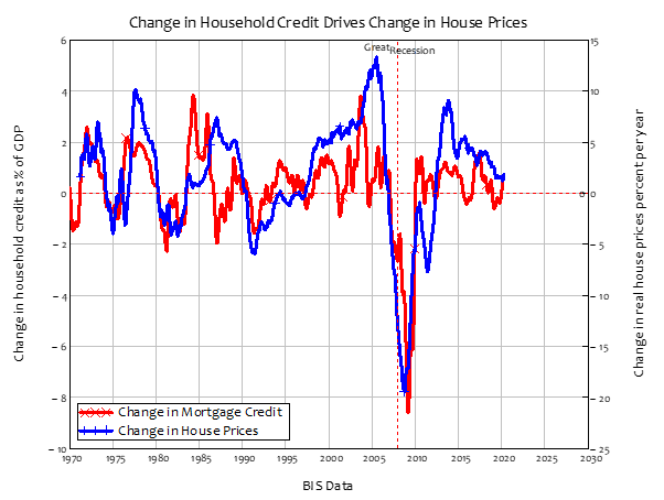
This type of borrowing drives asset price bubbles, and does precious little benefit to benefit society. We need means by which this kind of borrowing can be discouraged, while lending for productive purposed can be enhanced.

  1. “The Pill”

At present, if two individuals with the same savings and income are competing for a property, then the one who can secure a larger loan wins. This reality gives borrowers an incentive to want to have the loan to valuation ratio increased, which underpins the finance sector’s ability to expand debt for property purchases.

I instead propose basing the maximum debt that can be used to purchase a property on the income (actual or imputed) of the property itself. Lenders would only be able to lend up to a fixed multiple of the income-earning capacity of the property being purchased—regardless of the income of the borrower. A useful multiple would be 10, so that if a property rented for $30,000 p.a., the maximum amount of money that could be borrowed to purchase it would be $300,000.

Under this regime, if two parties were vying for the same property, the one that raised more money via savings would win. There would therefore be a negative feedback relationship between leverage and house prices: a general increase in house prices would mean a general fall in leverage. This would also encourage treating housing as it should be treated: a long-lived consumer good, rather than an object of speculation.

  1. Jubilee Shares

The key factor that allows Ponzi Schemes to work in asset markets is the “Greater Fool” promise that a share bought today for $1 can be sold tomorrow for $10. No interest rate, no regulation, can hold against the charge to insanity that such a feasible prospect foments. The vast majority of activity on the stock market is also the sale of existing shares by one speculator to another, which raises no capital for the company in question. The primary market—the sale of new shares by a company to raise capital—is trivial by comparison.

I propose the redefinition of shares in such a way that the enticement of limitless price appreciation can be removed, and the primary market can take precedence over the secondary market. A share bought in an IPO or rights offer would last forever (for as long as the company exists) as now, with all the rights it currently confers. It could be sold once onto the secondary market with all the same privileges. But on its next sale, it would have a life span of 50 years, at which point it would terminate.

The objective of this proposal is to eliminate the appeal of using debt to buy existing shares, while still making it attractive to fund innovative firms or startups via the primary market, and still making purchase of the share of an established company on the secondary market attractive to those seeking an annuity income.

I can envisage ways in which this basic proposal might be refined, while still maintaining the primary objective of making leveraged speculation on the price of existing share unappealing. The termination date could be made a function of how long a share was held; the number of sales on the secondary market before the Jubilee effect applied could be more than one. But the basic idea has to be to make borrowing money to gamble on the prices of existing shares a very unattractive proposition.

  1. Entrepreneurial Equity Loans

Entrepreneurs, in Schumpeter’s compelling vision of their role in capitalism’s development (Schumpeter 1934), are people with a good idea but no money with which to turn these ideas into products. Credit to entrepreneurs from banks is almost non-existent, though this function was the basis of Schumpeter’s explanation of the endogeneity of money. And for good reason: most entrepreneurs will fail, and banks that lend to them lose their capital, while only securing an interest-rate return from those entrepreneurs who succeed.

One way to encourage banks to lend to entrepreneurs in return for equity, rather than debt, via “Entrepreneurial Equity Loans” (EELs). Banks would still lose money on those entrepreneurs that failed, but could make a capital gain as well as a flow of dividends on those entrepreneurs who succeeded.

  1. Shifting the monetary paradigm

I am often asked what I would keep of Neoclassical economics in a new paradigm. My answer is that I would keep as much of Neoclassical economics as modern astronomy kept of Ptolemaic astronomy—which is to say, nothing at all. On its own, that answer may seem both arrogant and flippant: surely there is something of value in all the work done by Neoclassical economists?

There are skerricks of merit in the entire edifice. But I hope that is evident after this chapter on money that nothing of worth remains of the Neoclassical perspective on money and banking, once the reality that banks create money is accepted. Rather than being irrelevant to macroeconomics, banks, private debt, and money, are essential. Rather than playing no role in macroeconomics, credit is a significant component of aggregate demand and income, and, given its volatility, it is the “causa causans” (Keynes 1937, p. 221) that drives macroeconomics. Financial crises, rather than being “Black Swans”, are products of credit turning negative. Private debt, not government debt, is dangerous when it is high relative to GDP. Governments should normally run deficits to create identical surpluses for the non-government sectors. Government debt does not burden future generations but instead generates monetary assets for current ones. All the Neoclassical arguments about money are invalid: there is nothing at all to keep.

The same applies to the next, more technical failing of Neoclassical economics: its obsession with modelling the economy as if it has a stable equilibrium.

  1. References

Aristotle and H. D. P. L. (translator) (350 BCE [1952]). Meteorologica / Aristotle. London, Heinemann.

Bernanke, B. (2010). Aiding the Economy: What the Fed Did and Why. The Washington Post, The Washington Post.

Bernanke, B. S. (2000). Essays on the Great Depression. Princeton, Princeton University Press.

Census, B. o. (1949). Historical Statistics of the United States 1789-1945. B. o. t. Census. Washington, United States Government.

Census, B. o. (1975). Historical Statistics of the United States Colonial Times to 1970. B. o. t. Census. Washington, United States Government.

Chambers, C. (2019). “Bitcoin Really Is Money, Here’s Why.” Forbes
https://www.forbes.com/sites/investor/2019/02/15/bitcoin-really-is-money-heres-why/?sh=f01d78679d22.

Coolidge, C. (1928). State of the Union Address: Calvin Coolidge (December 4, 1928).

Coppola, F. (2019). People’s Quantitative Easing. Cambridge, Polity Press.

Deutsche Bundesbank (2017). “The role of banks, non- banks and the central bank in the money creation process.” Deutsche Bundesbank Monthly Report
April 2017: 13-33.

Fisher, I. (1929). Fisher sees stocks permanently high. New York Times. New York, New York Times. 16 October 1929.

Fisher, I. (1932). Booms and Depressions: Some First Principles. New York, Adelphi.

Fisher, I. (1933). “The Debt-Deflation Theory of Great Depressions.” Econometrica
1(4): 337-357.

Fontana, G. and R. Realfonzo, Eds. (2005). The Monetary Theory of Production: Tradition and Perspectives. Basingstoke, Palgrave Macmillan.

Fullwiler, S. T. (2013). “An endogenous money perspective on the post-crisis monetary policy debate.” Review of Keynesian Economics
1(2): 171–194.

Gleeson-White, J. (2011). Double Entry. Sydney, Allen and Unwin.

Graziani, A. (1989). “The Theory of the Monetary Circuit.” Thames Papers in Political Economy
Spring: 1-26.

Holmes, A. R. (1969). Operational Constraints on the Stabilization of Money Supply Growth. Controlling Monetary Aggregates. F. E. Morris. Nantucket Island, The Federal Reserve Bank of Boston: 65-77.

Ireland, P. N. (2011). “A New Keynesian Perspective on the Great Recession.” Journal of Money, Credit, and Banking
43(1): 31-54.

Keen, S. (1995). “Finance and Economic Breakdown: Modeling Minsky’s ‘Financial Instability Hypothesis.’.” Journal of Post Keynesian Economics
17(4): 607-635.

Kelton, S. (2020). The Deficit Myth: Modern Monetary Theory and the Birth of the People’s Economy. New York, PublicAffairs.

Keynes, J. M. (1937). “The General Theory of Employment.” The Quarterly Journal of Economics
51(2): 209-223.

Krugman, P. (2009). “Liquidity preference, loanable funds, and Niall Ferguson (wonkish).” The Conscience of a Liberal
http://krugman.blogs.nytimes.com/2009/05/02/liquidity-preference-loanable-funds-and-niall-ferguson-wonkish/.

Krugman, P. (2011). “Debt Is (Mostly) Money We Owe to Ourselves.” The Conscience of a Liberal
http://krugman.blogs.nytimes.com/2011/12/28/debt-is-mostly-money-we-owe-to-ourselves/ 2012.

Krugman, P. (2011). “Liquidity Preference and Loanable Funds, Still (Wonkish).” The Conscience of a Liberal
http://krugman.blogs.nytimes.com/2011/06/03/liquidity-preference-and-loanable-funds-still-wonkish/.

Krugman, P. (2012). End this Depression Now! New York, W.W. Norton.

Krugman, P. (2013). “Commercial Banks As Creators of “Money”.” The Conscience of a Liberal
http://krugman.blogs.nytimes.com/2013/08/24/commercial-banks-as-creators-of-money/.

Krugman, P. (2014). “A Monetary Puzzle.” The Conscience of a Liberal
http://krugman.blogs.nytimes.com/2014/04/28/a-monetary-puzzle/.

Krugman, P. (2015). “Debt Is Money We Owe To Ourselves.” New York Times
https://krugman.blogs.nytimes.com/2015/02/06/debt-is-money-we-owe-to-ourselves/?_r=0.

Krugman, P. (2015). “Debt: A Thought Experiment.” New York Times
https://krugman.blogs.nytimes.com/2015/02/06/debt-a-thought-experiment/.

Kumhof, M. and Z. Jakab (2015). Banks are not intermediaries of loanable funds — and why this matters. Working Paper. London, Bank of England.

Kumhof, M., R. Rancière and P. Winant (2015). “Inequality, Leverage, and Crises.” The American Economic Review
105(3): 1217-1245.

Mankiw, N. G. (2016). Macroeconomics. New York, Macmillan.

Marglin, S. A. and J. B. Schor (1992). Golden Age of Capitalism. Oxford, UK, Clarendon Press Oxford.

Marx, K. (1894). Capital Volume III. Moscow, International Publishers.

McLeay, M., A. Radia and R. Thomas (2014). “Money creation in the modern economy.” Bank of England Quarterly Bulletin
2014 Q1: 14-27.

McLeay, M., A. Radia and R. Thomas (2014). “Money in the modern economy: an introduction.” Bank of England Quarterly Bulletin
2014 Q1: 4-13.

Minsky, H. (1963). Can “It” Happen Again? Banking and Monetary Studies. D. Carson. Homewood, Richard D Irwin: 101-111.

Minsky, H. P. (1963). Can “It” Happen Again? Banking and Monetary Studies. D. Carson. Homewood, Illinois, Richard D. Irwin: 101-111.

Minsky, H. P. (1975). John Maynard Keynes. New York, Columbia University Press.

Minsky, H. P. (1977). “The Financial Instability Hypothesis: An Interpretation of Keynes and an Alternative to ‘Standard’ Theory.” Nebraska Journal of Economics and Business
16(1): 5-16.

Minsky, H. P. (1978). “The Financial Instability Hypothesis: A Restatement.” Thames Papers in Political Economy
Autumn 1978.

Minsky, H. P. (1982). Can “it” happen again? : essays on instability and finance. Armonk, N.Y., M.E. Sharpe.

Minsky, H. P. (1990). Longer Waves in Financial Relations: Financial Factors in the More Severe Depressions. Monetary theory. T. Mayer. Aldershot, U.K., Elgar: 352-363.

Minsky, H. P. and M. D. Vaughan (1990). “Debt and Business Cycles.” Business Economics
25(3): 23-28.

Mirowski, P. (2020). The Neoliberal Ersatz Nobel Prize. Nine Lives of Neoliberalism. D. Plehwe, Q. Slobodian and P. Mirowski. London, Verso: 219-254.

Modigliani, F. and H. M. Merton (1958). “The Cost of Capital, Corporation Finance and the Theory of Investment.” The American Economic Review
48(3): 261-297.

Moore, B. J. (1979). “The Endogenous Money Stock.” Journal of Post Keynesian Economics
2(1): 49-70.

Moore, B. J. (1988). Horizontalists and Verticalists: The Macroeconomics of Credit Money. Cambridge, Cambridge University Press.

Moore, B. J. (1997). “Reconciliation of the Supply and Demand for Endogenous Money.” Journal of Post Keynesian Economics
19(3): 423-428.

Moore, B. J. (2001). Some Reflections on Endogenous Money. Credit, interest rates and the open economy: Essays on horizontalism. L.-P. Rochon and M. Vernengo. Edward Elgar, Cheltenham: 11-30.

Offer, A. and G. Söderberg (2016). The Nobel Factor: The Prize in Economics, Social Democracy, and the Market Turn. New York, Princeton University Press.

Roberts, A. (2012). America’s first Great Depression: economic crisis and political disorder after the Panic of 1837. Ithaca, Cornell University Press.

Schumpeter, J. A. (1934). The theory of economic development : an inquiry into profits, capital, credit, interest and the business cycle. Cambridge, Massachusetts, Harvard University Press.

Sennholz, H. F., Ed. (1975). Gold is Money. London, Greenwood Press.

Taleb, N. N. (2010). The black swan : the impact of the highly improbable / Nassim Nicholas Taleb. London, London : Penguin.

Vague, R. (2019). A Brief History of Doom: Two Hundred Years of Financial Crises. Philadelphia, University of Pennsylvania Press.

Werner, R. A. (2014). “Can banks individually create money out of nothing? — The theories and the empirical evidence.” International Review of Financial Analysis
36(0): 1-19.

Werner, R. A. (2014). “How do banks create money, and why can other firms not do the same? An explanation for the coexistence of lending and deposit-taking.” International Review of Financial Analysis
36(0): 71-77.


Introduction to The New Economics: A Manifesto

I’m writing a book for Polity Press entitled The New Economics: A Manifesto. It has a long way to go, but this is the reasonably complete first chapter.

  1. Why this Manifesto?

Even before the Covid-19 crisis began, the global economy was not in good shape, and nor was economic theory. The biggest economic crisis since the Great Depression began late in first decade of the 21st century. Called the “Global Financial Crisis” (GFC) in most of the world and the “Great Recession” in the USA, it saw unemployment explode from 4.6% of the US workforce in early 2007 to 10% in late 2009. Inflation turn into deflation— inflation of 5.6% in mid-2008 fell to minus 2% per year in mid-2009—and the stock market collapsed, with the S&P500 Index falling from 1500 in mid-2007 to under 750 in early 2009. The economy recovered very slowly after then, under the influence of an unprecedented range of government interventions, from the “cash for clunkers” scheme that encouraged consumers to dump old cars and buy new ones, to “Quantitative Easing”, where the Federal Reserve purchased a trillion-dollars-worth of bonds from the financial sector every year, in an attempt to stimulate the economy by making the wealthy wealthier.

This crisis surprised both the policy economists who advise governments on economic policy, and the academic who develop the theories and write the textbooks that train the vast majority of new economists. They had expected a continuation of the boom conditions that had preceded the crisis, and they in fact believed that crises could not occur. In his Presidential Address to the American Economic Association in January 2003, Nobel Prize winner Robert Lucas declared that crises like the Great Depression could never occur again because “Macroeconomics … has succeeded: Its central problem of depression prevention has been solved, for all practical purposes, and has in fact been solved for many decades. (Lucas 2003 , p. 1 ; emphasis added). Just two months before the crisis began, the Chief Economist of the Organization for Economic Cooperation and Development (OECD), the world’s premier economic policy body, declared that “the current economic situation is in many ways better than what we have experienced in years“, and predicted that “sustained growth in OECD economies would be underpinned by strong job creation and falling unemployment.” (Cotis 2007 , p. 7; emphases added)

How could they be so wrong? Economists could be excused for this failure to see the Great Recession coming if the crisis were something like Covid-19, when a new pathogen suddenly emerged out of China. That such a plague would occur was predicted as long ago as 1995 (Garrett 1995). But predicting when the pathogen would emerge, let alone what its characteristics would be, was clearly impossible. However, the epicentre of the Great Recession was the US financial system itself: the crisis came from inside the economy, rather than from outside. Surely there were warning signs? As Queen Elizabeth herself put it when she attended a briefing at the London School of Economics in 2008, “If these things were so large, how come everyone missed them?” (Greenhill 2008).

Not all economists did: there were some who warned that a crisis was not merely likely, but imminent. The Dutch economist Dirk Bezemer identified a dozen, of whom I was one (Keen 1995; Keen 2007; Bezemer 2009; Bezemer 2009; Bezemer 2010). Though these economists came from disparate backgrounds, Bezemer noted that they had one negative characteristic in common: “no one predicted the crisis on the basis of a neo-classical framework” (Bezemer 2010, p. 678).

“Neoclassical” economics is the method of thinking about and modelling the economy that the majority of economists use today—both Lucas and the OECD Chief Economist (then and now) are Neoclassical economists. For this reason, it is often also called “mainstream economics”. But it is not the only framework. Though the Neoclassical approach has dominated the discipline since the 1870s, it has never completely replaced previous approaches to economics, and rival approaches to it have developed since the 1870s.

These rival approaches in economics are very different to divisions of thought in sciences like physics. Albert Einstein’s General Relativity and Max Planck’s Quantum Mechanics have supplanted Isaac Newton’s physics in the realms of the very large (the Universe) and very small (the atom), but in between, Newton’s equations work very well. They are fundamentally different visions of the how the Universe operates, but anyone who rejects any of these approaches in physics in their relevant realm is highly likely to be a “crank”, who could never get a position in an academic physics department.

But in economics, different schools of thought have visions of how the economy works that are fundamentally in conflict. There is no way to partition the economy into sections where Neoclassical economics applies and others where Austrian, Marxian or Post Keynesian theory applies. On the same topic—say, for example, the role of private debt in causing financial crises—these schools of thought will have answers that flatly contradict each other.

Economists who do reject the mainstream, the so-called “heterodox” economists, also make up a significant minority of academic economists—as much as 1/6th of the discipline, going on a campaign by French academic economists in 2015 to establish a separate classification there (Lavoie 2015; Orléan 2015). So there is something fundamentally incompatible between the Neoclassical and heterodox approaches to economics, and the heterodox economists cannot be dismissed as cranks.

The common themes that Bezemer identified in the work of those who warned of the Global Financial Crisis indicate one of the key incompatibilities. Mainstream macroeconomic models ignore banks, debt, and money (Bezemer 2010, p. 678), while most heterodox economists regard banks, debt and money as crucial concepts in economics.

If you haven’t yet studied economics, or you’re in your early days of doing so at school or university, I hope this gives you pause: “Neoclassical economics doesn’t concern itself with money? But isn’t economics about money?” I, and many other heterodox economists, would respond “Yes, it is!”. But the mainstream long ago convinced itself that money doesn’t really affect the economy, and hence monetary phenomena are omitted from Neoclassical models. One Neoclassical economist put it this way on Twitter:

Most people who teach macro do it by leading people through simple models without money, so they understand exchange and production and trade, international and inter-temporal. You can even do banks without money [yes!]. And it’s better to start there. Then later, study money as it superimposes itself and complicates things, giving rise to inflation, exchange rates, business cycles.

Figure 1: Tony Yates defending moneyless macroeconomics on Twitter on October 19th 2020

This statement was made in late 2020—a dozen years after the failure of Neoclassical models to anticipate the crisis.

Why didn’t mainstream economists change their beliefs about the significance of money in economics after their failure in 2007? Here, paradoxically, economics has been like physics, in that significant change in physics does not, in general, occur because adherents of an old way of thinking become convinced by an experiment whose results contradicted their theory. Instead, these adherents continued to cling to their theory despite the experimental evidence it had failed. Humans, it appears, are more wedded to their beliefs about reality—their “paradigms”, to use Thomas Kuhn’s famous phrase (Kuhn 1970)—than reality itself. Science changed, not because these scientists changed their minds, but because they were replaced by new scientists who accepted the new way of thinking. As Max Planck put it:

“a new scientific truth does not triumph by convincing its opponents and making them see the light, but rather because its opponents eventually die, and a new generation grows up that is familiar with it.” (Planck 1949, pp. 33-34)

Here, economics is different, largely because economic truths are different to scientific ones in that they are historical, whereas scientific truths are unchanging. The key scientific experiment that led to Einstein’s theory of relativity was the Michelson-Morley experiment in 1887, which attempted to measure the speed of the Earth relative to “the aether”, the medium that scientists then thought allowed light to travel through space. Michelson and Morley’s experiments found that there was no discernible relative motion—which implied that the aether did not exist. This experiment can be repeated at any time—and has been repeated, with increasingly more sophisticated methods—and the result is always the same. There is no way of getting away from it and returning to a pre-Relativity science—nor is there any desire to do so by post-Relativity physicists.

In economics, it is possible to get away from failures of theory to play out as expected in reality. An event like the GFC occurs only once in history, and it cannot be reproduced to allow old and new theories to be tested against it. As time goes on, the event itself fades from memory. History can help sustain a memory, but economic history is taught at very few universities. Economics don’t learn from history because they’re not taught it in the first place.

Economics is also a moving target, whereas physics, relatively, is a stationary one. When a clash between theoretical prediction and empirical results occurs in physics, the state of unease persists until a theoretical resolution is found. But in economics, though a crisis like the GFC can cause great soul searching at the time, the economy changes over time, and the focus of attention shifts.

Finally, unlike physicists, economists do want to return to pre-crisis economic theory. Events like the GFC upset the totem that characterises Neoclassical economics, the “supply and demand” diagram, in which the intersecting lines determining both equilibrium price and equilibrium quantity, and in which any outside intervention necessarily makes things worse by moving the market away from this equilibrium point. This image of a self-regulating market system that always returns to equilibrium after an “exogenous shock” is a powerful emotional anchor for mainstream economists.

These factors interact to make economics extremely resistant to fundamental change. In physics, anomalies like the clash between the results of the Michelson-Morley experiment and the predictions of pre-Relativity physics persist until the theory changes, because the experimental result is eternal. The anomaly doesn’t go away, but the theory that it contradicted dies with the pre-anomaly scientists, who can’t recruit followers amongst new students, because they are aware of the anomaly, and won’t accept any theory that doesn’t resolve it.

In economics, anomalies are forgotten, and new students can be recruited to preserve and extend the old beliefs to cover new phenomena. School and university economics courses become ways of reinforcing the Neoclassical paradigm, rather than fonts from which new theories spring in response to failures of the dominant paradigm.

This means that intellectual crises in physics are intense but, to some extent, short-lived. The crisis persists until a new theoretical breakthrough resolves it—regardless of whether that breakthrough persuades existing physicists (which as a rule, it doesn’t). The “anomaly”, the empirical fact that fundamentally contradicts the existing paradigm, is like the grain of sand in an oyster that ultimately gives birth to a pearl: the irritation cannot be avoided, so it must be dealt with. It is the issue that believers in the existing paradigm know they cannot resolve—though it may take time for that realisation to sink in, as various extensions of the existing paradigm are developed, each of which proves to be partially effective but inherently flawed. It is the thing young scientists are most aware of, the issue they want to be the one to resolve. As their lecturers who stick to the old paradigm age, the students take in the old ideas, but are actively looking for where they are wrong, how these contradictions might be resolved.

Once a solution is found, the protestations of the necessarily older, aged and often retired champions of the previous paradigm, mean nothing. Ultimately, all the significant positions in a university department are filled by scientists who are committed to the new paradigm.

As that is pushed further, then, as philosopher of science Thomas Kuhn (Kuhn 1970) explains, the new paradigm undergoes a period of rapid extension just like its predecessor, but ultimately this new paradigm will confronts its own critical anomaly, and the science falls into crisis once more.

This is a punctuated path of development. It starts with the development of an initial paradigm by a great thinker, around whom a community of followers develop. They extend the core insights and thus form a science, and initially enjoy a glorious period of the dance between observation and theory, where observations confirm and extend the paradigm. But finally, some prediction the theory makes is contradicted by observation. After a period of denial and dismay, the science settles into an unhappy peace: the paradigm is taught, but with less enthusiasm, the anomaly is noted, and the various withing-paradigm attempts to resolve it are discussed. Then, out of somewhere, whether from a Professor (Planck) or a patents clerk (Einstein), a resolution comes. Rinse and repeat.

Those punctuations never occur in economics, and because the punctuations don’t occur, neither does the kind of revolutionary change in the discipline that Kuhn vividly describes for physics and astronomy.

An economic crisis, when it strikes, does disturb the mainstream. Their textbook advice—if the crisis is empirical rather than theoretical—is thrown out the window by policymakers while the crisis lasts. But mainstream economists react defensively. They justify the extraordinary measures by the unexpected nature of the crisis, then treat the contradiction the crisis poses for their theory as an aberration, which can be handled by admitting some modifications to the core theory. One example is the concept of “bounded rationality” promoted by Joe Stiglitz (Stiglitz 2011; Stiglitz 2018). This can be invoked to say that, if everyone were strictly rational, then no problem would arise, but because of “bounded rationality”, the general principle doesn’t apply and, in this instance, a deviation from the theoretical canon is warranted.

Minor modifications are made to the core Neoclassical paradigm, but fundamental aspects of it remain sacrosanct.

Over time, the crisis passes—whether that was aided or hindered by the advice of economists. A handful of economists break with the majority, which is how heterodox economists are born. But the majority of students become as entranced as their teachers were by the fundamentally utopian vision of Neoclassical economics—a world without power, in which everyone receives their just rewards, and in which regulation and punishment are unnecessary, because The Market does it all. These new students replace their masters, and they continue to propagate the Neoclassical paradigm.

That fraction which breaks away—the roughly one in six academic economists who refuse to ignore the crisis, reject the mainstream, and then get attracted to a competing paradigm (like Post Keynesian, Marxian or Austrian Economics)—live on in universities, but don’t get the positions, promotions or research funds that accrue to the true believers in Neoclassical economics. Instead, they get positions in lowly ranked universities which leading Neoclassicals aren’t interested in—like the University of Western Sydney, and Kingston University London, where I was respectively a Professor and Head of School, or in Departments of Business or Management. The influence of heterodox economists is limited, but they exist at all times.

Given this failure to break the dominant Neoclassical paradigm despite numerous crises, both empirical and logical (Keen 2011), the discipline sits in a state of perpetual and understated crisis: a minority of heterodox economists vocally reject the Neoclassical mainstream, but the Neoclassical paradigm remains dominant. It evolves over time, but it is never replaced in the way that obsolete paradigms are replaced in science.

If you’re thinking “But what about the Keynesian revolution?”, that was snuffed out by John Hicks, with a paper that purported to reach a reconciliation between “Mr Keynes and the Classics” (Hicks 1937) by developing what became known as the IS-LM model. Though this model was presented and accepted by the majority of economists as “a convenient synopsis of Keynesian theory”, Hicks later admitted that it was a Neoclassical, “general equilibrium” model he had sketched out “before I wrote even the first of my papers on Keynes” (Hicks 1981, p. 140).

The gap between what this model alleged was Keynesian economics, and the actual economics of Keynes, was enormous, as can readily be seen by comparing Hicks’s “suggested interpretation” of Keynes, and Keynes’s own 24-page summary of his economics in “The General Theory of Employment” (Keynes 1937), which was published 2 months before Hicks’s paper. The key passage in Keynes’s summary is the following:

The theory can be summed up by saying that … the level of output and employment as a whole depends on the amount of investment… More comprehensively, aggregate output depends on … But of these several factors it is those which determine the rate of investment which are most unreliable, since it is they which are influenced by our views of the future about which we know so little.

This that I offer is, therefore, a theory of why output and employment are so liable to fluctuation. (Keynes 1937, p. 221. Emphasis added)

Keynes model sees the level of investment as depending primarily upon investors’ expectations of the future, which are uncertain and “unreliable”. Hicks completely ignored expectations—let alone uncertainty—and instead, modelled investment as depending upon the money supply and the rate of interest:

This brings us to what, from many points of view, is the most important thing in Mr. Keynes’ book. It is not only possible to show that a given supply of money determines a certain relation between Income and interest…; it is also possible to say something about the shape of the curve. It will probably tend to be nearly horizontal on the left, and nearly vertical on the right…

Therefore, … the special form of Mr. Keynes’ theory becomes valid. A rise in the schedule of the marginal efficiency of capital only increases employment, and does not raise the rate of interest at all. We are completely out of touch with the classical world. (Hicks 1937, p. 154)

The schism between Hicks’s Neoclassical purported model of Keynes and Keynes’s own views was so great that it gave rise to one of the key heterodox schools of thought, “Post Keynesian Economics”. So “the Keynesian revolution” didn’t happen, though Post Keynesians themselves—including myself (Keen 2020)—have developed approaches to economics that are revolutionary. But a revolution in thought, like that from Ptolemy’s earth-centric vision of the solar system to Copernicus’s sun-centric vision, has not happened.

The above paints a bleak picture of the prospects of replacing Neoclassical economics with a fundamentally different and far more realistic paradigm. But there have been changes over time that make this more feasible now than it was at Keynes’s time.

Foremost here is the development of the computer, and computer software that can easily handle large scale dynamic and even evolutionary processes. These developments have occurred outside economics, and especially in engineering, physics and meteorology. There are limitations of the applicability of these techniques to economics, largely because of the fact that economics involves human behaviour rather than the interaction of unconscious objects, but as I will argue in the following chapters, these limitations distort reality far less than the Neoclassical fantasy that economic processes occur in or near equilibrium.

The development of the Post Keynesian school of thought after the Great Depression is also important. There were strident critics of the Neoclassical mainstream before the Great Depression, such as Thorstein Veblen (Veblen 1898; Veblen 1908; Veblen 1909), but no truly revolutionary school of economic thought. The development of this heterodox school over the 8 decades between the Great Depression and the GFC meant that, when that crisis struck, there were coherent explanations of it—indeed, prescient warnings of it (Keen 1995; Godley and Wray 2000; Godley 2001; Godley and Izurieta 2002; Keen 2006; Keen 2007)—that did not exist when Keynes attempted his revolution.

Social media has also allowed student movements critical of Neoclassical economics to evolve, flourish and persist in a way that was impossible before the Internet. I led the first student revolt against Neoclassical economics at Sydney University in 1973 (Butler, Jones et al. 2009), but that was restricted to just one university in far-away Australia. French students established the “Protest Against Austistic Economics” in 2000, which had somewhat more traction, but whose main legacy was an online journal called the Real World Economic Review. The real breakthrough came with a protest by economics students at the University of Manchester in the UK in 2012, in response to the failure of their teachers to take the GFC seriously in their macroeconomics courses. As they put it, “The economics we were learning seemed separate from the economic reality that the world was facing, and devoid from the crisis that had made many of us interested in economics to begin with”. Their Post Crash Economics movement in turn spawned the international Rethinking Economics campaign, which now has groups in about 100 universities across the world.

There are therefore students eager for approaches to economics that break away from the Neoclassical mainstream, methods of analysis which can easily supplant the dated equilibrium methods used by Neoclassical economics, and rival schools of thought with an intellectual tradition spanning 70 years on which an alternative paradigm can be constructed. What we lack is a university system in which these conditions can foment change as occurs in physics.

Hence this Manifesto: I want to reach potential students of economics before they embark on a university course of study that will attempt to inculcate belief in the Neoclassical paradigm, and that will drive away those that can’t accept it.

  1. Appendix

  1. References

    Bezemer, D. J. (2009). “‘No one saw this coming’ – or did they?” VOX EU, from https://voxeu.org/article/no-one-saw-coming-or-did-they.

    Bezemer, D. J. (2009). “No One Saw This Coming”: Understanding Financial Crisis Through Accounting Models. Groningen, The Netherlands, Faculty of Economics University of Groningen.

    Bezemer, D. J. (2010). “Understanding financial crisis through accounting models.” Accounting, Organizations and Society
    35(7): 676-688.

    Butler, G., E. Jones, et al. (2009). Political Economy Now!: The struggle for alternative economics at the University of Sydney. Sydney, Darlington Press.

    Cotis, J.-P. (2007). Editorial: Achieving Further Rebalancing. OECD Economic Outlook. OECD. Paris, OECD. 2007/1: 7-10.

    Garrett, L. (1995). The coming plague : newly emerging diseases in a world out of balance / Laurie Garrett. New York, New York : Penguin Books USA Inc.

    Godley, W. (2001). “The Developing Recession in the United States.” Banca Nazionale del Lavoro Quarterly Review
    54(219): 417-425.

    Godley, W. and A. Izurieta (2002). “The Case for a Severe Recession.” Challenge
    45(2): 27-51.

    Godley, W. and L. R. Wray (2000). “Is Goldilocks Doomed?” Journal of Economic Issues
    34(1): 201-206.

    Greenhill, S. (2008). ‘It’s awful – Why did nobody see it coming?’: The Queen gives her verdict on global credit crunch. Mail Online. London.

    Hicks, J. (1981). “IS-LM: An Explanation.” Journal of Post Keynesian Economics
    3(2): 139-154.

    Hicks, J. R. (1937). “Mr. Keynes and the “Classics”; A Suggested Interpretation.” Econometrica
    5(2): 147-159.

    Keen, S. (1995). “Finance and Economic Breakdown: Modeling Minsky’s ‘Financial Instability Hypothesis.’.” Journal of Post Keynesian Economics
    17(4): 607-635.

    Keen, S. (2006). Steve Keen’s Monthly Debt Report November 2006 “The Recession We Can’t Avoid?”. Steve Keen’s Debtwatch. Sydney. 1: 21.

    Keen, S. (2007). Deeper in Debt: Australia’s addiction to borrowed money. Occasional Papers. Sydney, Centre for Policy Development.

    Keen, S. (2011). Debunking economics: The naked emperor dethroned? London, Zed Books.

    Keen, S. (2020). “Emergent Macroeconomics: Deriving Minsky’s Financial Instability Hypothesis Directly from Macroeconomic Definitions.” Review of Political Economy
    32(3): 342-370.

    Keynes, J. M. (1937). “The General Theory of Employment.” The Quarterly Journal of Economics
    51(2): 209-223.

    Kuhn, T. (1970). The Structure of Scientific Revolutions. Chicago, University of Chicago Press.

    Lavoie, M. (2015). “Should heterodox economics be taught in economics departments, or is there any room for backwater economics?” INET Economics https://www.ineteconomics.org/uploads/papers/Lavoie.pdf.

    Lucas, R. E., Jr. (2003). “Macroeconomic Priorities.” American Economic Review
    93(1): 1-14.

    Orléan, A. (2015). Economists also need competition. Le monde. Paris.

    Planck, M. (1949). Scientific Autobiography and Other Papers. London, Philosophical Library; Williams & Norgate.

    Stiglitz, J. E. (2011). “Rethinking Macroeconomics: What Failed, and How to Repair It.” Journal of the European Economic Association
    9(4): 591-645.

    Stiglitz, J. E. (2018). “Where modern macroeconomics went wrong.” Oxford Review of Economic Policy
    34(1-2): 70-106.

    Veblen, T. (1898). “Why is Economics not an Evolutionary Science?” THE QUARTERLY JOURNAL OF ECONOMICS
    12(4): 373-397.

    Veblen, T. (1908). “Professor Clark’s Economics.” THE QUARTERLY JOURNAL OF ECONOMICS
    22(2): 147-195.

    Veblen, T. (1909). “The Limitations of Marginal Utility.” The Journal of Political Economy
    17(9): 620-636.


Personal reflections on dumping Trump from an ex-victim of a Narcissist

There is a set of people with a special, personal perspective on Trump: those who have had, and survived, a relationship with a Narcissistic Personality Disorder… sufferer isn’t the right word, because they cause far more suffering than they ever feel.

I had a relationship with a NPD … perpetrator … in the early 2000s (the relationship began on September 11 2001, but that’s another story). There were some good things about that relationship as well as bad, but the one thing I can say emphatically in favor of it in hindsight, is that it gave me deep insights into Donald Trump.
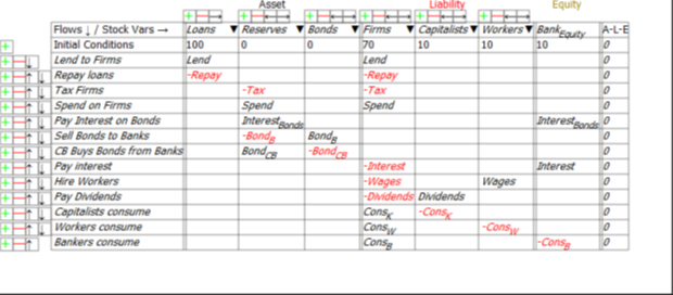
The deepest insight that one gets about a Narcissist from knowing one intimately is that they neither lie, nor tell the truth. Instead, everything they say is a reconstruction of what has happened so that they are always in the right. “Truth” and “Lie” are concepts that require an internal frame of reference to an objective external reality. They don’t have that framework: instead, their frame of reference is themselves. Everything must start and end with them as the center of attention, and with them acting correctly throughout.

So, when reality doesn’t follow that narrative, as it inevitably does not, they reverse engineer reality until it fits that narrative.

I’ll give my favourite illustration of that from my relationship. I won’t use her real name (though anyone who’s known me personally or professionally for more than 15 years knows who I’m talking about): instead, I’ll call her Aida.

We were at a conference celebrating the life work of the great, and now sadly departed, Basil Moore, in Cape Town, South Africa. The food and wine at the restaurants in Cape Town, Stellenbosch and surrounds, was beyond excellent, and in overindulging, I developed pimples on my neck.

Aida had, as usual, made enemies of the other female attendees. In talking with two of them one morning, one quipped, in reference to the red welts on my neck, “Steve, it looks like you slept with a vampire last night”.

In an attempt to make light of that very clever snipe, I replied “Ah, but she isn’t a vampire, she’s a vamp”.

Before the other two women had a chance to react, Aida snarled at me “How dare you call me a slut in front of these women Steve!”

I replied “But Aida, vamp doesn’t mean slut!”. “Yes it does Steve, it means it in every language. I’m grossly offensed.” (English was not her first language).

Since this was easily the hundredth time she’d abused me in public, I replied “Well, be offensed then, just leave me alone!” and stormed off.

Round two.

Back at her home after the conference, I remembered her telling one of my sisters that, when she heard English, she first translated into French and then her own language before replying. Whether that was true or not, it left open the possibility that she had misinterpreted the word “vamp” as something derogatory. So, I asked her “Aida, when I said vamp, did you hear something like prostitute?”

“Yes, I did Steve!”, she replied, visibly overjoyed that I understood her.

“But that’s not what it means, Aida”.

“But that’s what I learnt that it meant. Look, I’ll show you”, and she went to her bookshelf to retrieve an ancient English dictionary.

As I say next to her so that we could both read the entry, she turned to the relevant page, and there was the definition of Vamp.

It was, and I quote, “sophisticated and irresistible woman“—precisely the meaning I meant to convey.

She went silent. No apology, no discussion.

Round three

By this time, I had already decided to leave her—the only questions were when, and how. So, when we went for dinner that night, I had just one thought on my mind: “before I leave, I’m going to get an apology out of this bitch if it kills me”. I thought I had the perfect chance with this event.

But, as I went to raise the issue, Aida snarled at me from across the table:

“Yes Steve, and the other women we were talking to weren’t attractive enough to be vamps, and I was offensed on their behalf.”

It didn’t matter that this was blatantly untrue. It didn’t matter that I was there, and knew it was untrue. All that mattered was that, in the light of new evidence (her dictionary), she now had a new narrative that put her, once more, in the right throughout.

So, everything that Trump has done, from the claim that his inauguration crowd was the biggest in history, to the claim he won the election against Biden, to—finally and rather pathetically– him consoling himself with the fact that he got more votes than any previous sitting President, made perfect sense to me. It was simply his NPD perspective on everything.

My worry now is what will he do for the next two months before, under the ludicrously complicated US political system, he finally ceases being President.

The best outcome, I think, would be that he falls into a deep depression—which is feasible, since his NPD mind won’t be able to cope with the fact that, whatever he believes, he will cease being President on January 20. That will mean inaction, rather than vengeance. He will do the odd thing to make himself feel better—like sack Fauci—but otherwise, it will be inaction and neglect.

But if he shifts to vengeance? While still in command of the most powerful nation on Earth? Then I just hope those who enabled his dysfunctional behavior for so long will finally have the courage, now that his term is limited, to invoke the 25th amendment and remove him from office.

More likely of course, he will recover from the funk and begin the “I was robbed!” narrative that will be his ultimate consolation, and the foundation of his attempt to establish his own Trump-wing TV network for his post-Presidential career.

So we’ll never be fully free of him, but at least we can breathe a sigh of relief that his days of getting his NPD centre-of-attention hit in the role of President are over. And we can relish the schadenfreude as we say to him:

Donald Trump, you’re fired!

Preface to the Spanish Edition of Can we avoid another financial crisis?

As I write these words, Spain is suffering from its second wave of Covid-19, and it ranks 7th in the world for Covid-19 cases, when its rank in world population is far lower. It has, and is, experiencing more than its fair share of pain from the novel coronavirus.

Spain suffered far more than its fair share of pain during the Global Financial Crisis too. There is now a terrible danger that these two crises will compound each other, because neither Spain nor the rest of the world had truly recovered from the financial crisis when Covid-19 began.

I use the USA for most of my examples in this book, but in many ways Spain is a textbook example of the economic forces that caused the Global Financial Crisis (GFC), and how conventional economic thinking—epitomized most dramatically in the European Union’s limits on government debt and government deficits—helped cause the crisis, and made its impact even worse.

The data on Spain’s crisis and its bungled aftermath are so obvious that you might wonder why the thesis I defend in this book—that economic crises are caused not by government debt, but by private debt—is not the conventional wisdom. The role of Euro in triggering the boom in private debt, and thus making a crisis more likely, is also obvious. After an exciting first eight years, the Euro and its “Growth and Stability Pact” have led to contraction and instability.

Much was made of Spain’s success in meeting the Growth and Stability Pact’s target of government debt being below 60% of GDP. Government debt was 70% of GDP when the Euro commenced in 1999, and it fell to a low of 35% of GDP by mid-2008. It was almost the only country in the Euro to meet and exceed both of the Euro’s policy targets: a government debt level of less than 60% of GDP, and a deficit of less than 3% of GDP. In fact, it exceeded the deficit target handsomely, running not a merely a small deficit, but a substantial surplus between 2004 and the crisis, peaking at 2.5% of GDP in mid-2006—see Figure 1.

If the Euro’s rules had the effect they were intended to have, this should have meant that Spain was less likely to experience a crisis, and well prepared to handle it if one did occur. This proved to be the opposite of the truth.

Figure 1

The reason is starkly evident in Figure 2: while Spain was lauded for halving its level of Government debt, across the same time span, private debt almost trebled—and throughout, it dwarfed government debt. Private debt had no trend before the introduction of the Euro: it was 67% of GDP in 1970, rose as high as 85% in 1977, but by the start of the Euro, it had risen not at all: it was also 85% of GDP in 1999.

However, from the introduction of the Euro until 2010, it rose far more rapidly than government debt fell: as government debt fell by 35% of GDP, private debt rose by 140%.

Figure 2: Spanish Debt Levels

As I explain in this book, private debt drives economic performance, because the change in private debt—which I call credit, using the terminology of accounting—is a significant, and by far the most volatile, source of aggregate demand. It is therefore the dominant determinant of whether the economy will be in a boom or in a slump. And a credit-driven boom will contain the seeds of its own destruction in a crash, as I explain in this book.

While the Spanish government sector did what conventional wisdom regards as the right thing—reducing its debt by “living within its means”—the Spanish private sector did the opposite. It spent far more than it earned, and made up the difference with credit. This caused a credit-based boom in aggregate demand, which was a major reason why the government could run a surplus of as much as 2.5% of GDP per year at the same time. The government mistakenly attributed the economy’s strong performance in 2000-2007 to its surplus, but the real source of Spain’s boom was the growth of credit, from zero in 1995, to 10% of GDP when the Euro began, to a peak of 35% of GDP in 2008—almost 15 times the size of the government’s surplus.

Figure 3

That huge credit-debt-driven stimulus to demand came at a price: a huge increase in Spain’s private debt, from 80% of GDP when the Euro commenced, to 210% when the financial crisis began—see Figure 4.


Figure 4

Both the household and corporate sector indulged in the debt bubble—though the impact of the Euro was more marked on bank lending to the corporate sector than to households. The household sector doubled its debt level from the start of the Euro till the crisis, while corporate borrowing almost trebled.

Figure 5

The crisis began when credit started falling—a pattern which was repeated across the world, but was extremely obvious in Spain. When credit goes up, unemployment goes down, and vice versa, as Figure 6 illustrates.

Figure 6

You might wonder, if the relationship is this strong and this obvious, the why did the government do nothing about it?

It is largely because their economic advisors, who are trained in mainstream economics, learn a model of banking in which credit plays no significant role in macroeconomics. That model, known as “Loanable Funds”, is technically false, as the Bank of England explained in 2014 (Michael McLeay et al., 2014). A false theory can play the role of blinkers on a horse, stopping you from looking at data that contradicts it, like Figure 6. That data makes it abundantly clear that the mainstream theory is wrong—but the mainstream didn’t pay any attention to that data before the GFC, and it hasn’t altered its model of banking since. Mainstream economics textbooks continue to teach the same false model of banking, even after being told, not only by the Bank of England but also by the Bundesbank (Deutsche Bundesbank, 2017), that this model is wrong.

What even mainstream thinkers can’t deny is that bank lending drove a bubble in Spanish house prices, which had been falling before the Euro, but rose dramatically under its influence, doubling between the start of the Euro and the crisis.


Figure 7

The link between household debt and house prices is not obvious: in Figure 7, the price index rises as the debt level rises from 1999 till the GFC, and falls as debt falls until 2014, but from then on, house prices are rising while debt is still falling. However, as I explain in this book, the real causal link is between change in household credit, and change in house prices. As Figure 8 indicates, this link holds across all of the data, from well before the Euro commenced until today.

Figure 8

Spain’s boom under the Euro prior to the GFC was caused by a private debt bubble, its crisis was caused by that bubble bursting, and the limits on government spending imposed by the rules of the Euro made its decline worse. The economy only recovered when its period of negative credit—which reduces aggregate demand—came to an end. But that period lasted almost a decade, and was far deeper than in the USA, where the maximum level of negative credit was 5.3% of GDP, versus 20% for Spain.

Private debt was still too high after the crisis, at 150% of GDP, versus roughly 80% of GDP for the 30 year. That alone was a problem without Covid-19. With it, the financial consequences of Covid-19 could be as great as its health consequences. The Covid-19 crisis has drastically exacerbated the impact of being highly levered. Laid-off workers are not able to pay their rent or mortgage without government support, landlords lose the cash flow to service their mortgages, corporations are forced into short-term debt where they have access to it to make up for diminished cash flow, and many corporations have gone and will go bankrupt, undermining the viability of the banks which lent to them. Government policies have reduced the impact to some extent, but the pressure of pre-Covid-19 financial commitments on a post-Covid-19 world are a major reason why there has been so much political opposition to the lockdown measures used to constrain the virus’s spread.

In this light, a proposal I make in the book is now needed much more. A “Modern Debt Jubilee” (see pages 117-119) would use the State’s limitless capacity to create money to reduce private debt significantly—by as much as 100% of GDP. But an essential aspect of that policy is that government has both a Treasury and a Central Bank that can together create its currency. Because of the Euro, Spain does not have that—nor does any other member of the Euro. I therefore believe that, unless there is a drastic change of not only heart but thinking at the ECB and the upper levels of European politics, the Euro in particular—and European economic policy in general—is a hindrance to managing the twin crises of private debt and Covid-19.


Deutsche Bundesbank. 2017. “The Role of Banks, Non- Banks and the Central Bank in the Money Creation Process.” Deutsche Bundesbank Monthly Report, April 2017, 13-33.

McLeay, Michael; Amar Radia and Ryland Thomas. 2014. “Money Creation in the Modern Economy.” Bank of England Quarterly Bulletin, 2014 Q1, 14-27.


One Mathematical Model Of Modern Monetary Operations

This post collates three previous posts on modelling the domestic financial aspects of Modern Monetary Theory. There is a PDF of this post attached on my Patreon page, to aid offline reading. The Minsky model is also attached, and Minsky (which is free and Open Source) can be downloaded from https://sourceforge.net/projects/minsky/. This model uses features that are not in the current release version (version 2.18) so if you wish to run it, and 2.18 is still the release version, please download the latest beta version instead from https://sourceforge.net/projects/minsky/files/beta%20builds/.

I confess immediately that I chose the title because its acronym is a palindrome.

This model considers only the monetary aspects of MMT: the Job Guarantee and inflation management components are not yet incorporated. International trade and financial flows are not considered. However, the assertions of MMT about domestic monetary dynamics remain in dispute in economic and political circles, so it is worth putting these into a mathematical model where their veracity can be tested.

The primary stimulus for developing the model was the publication of Stephanie Kelton’s The Deficit Myth. Stephanie has written the book for non-technical readers, and she’s done a very good job: it’s a very easy read that explains why many conventional wisdoms about government spending are wrong. But MMT is facing heavy resistance in political and economic circles, with my favourite to date being a motion before the US Congress, posted by Representative Kevin Hern, to resolve:

That the House of Representatives (1) realizes that deficits are unsustainable, irresponsible, and dangerous; and (2) recognizes— (A) that the implementation of Modern Monetary Theory would lead to higher deficits and higher inflation; and (B) the duty of the House of Representatives to condemn Modern Monetary Theory.

The objective of this series of posts is to allow the assessment of the first part of this motion—the assertion that “deficits are unsustainable, irresponsible, and dangerous”.

The models in this document are built in the Open Source system dynamics program Minsky, whose unique feature is the capacity to build models of financial flows using what are called Godley Tables (in honour of Wynne Godley, the pioneer of stock-flow-consistent-modelling). These tables enforce the “law of accounting” that (see Figure 1).

Figure 1: A blank Godley Table

Once an account is flagged as an “Asset” for one entity, Minsky knows that it has to also be shown as a “Liability” for another entity. This
makes it possible to take an integrated look at the financial system, which allows us to assess Hern’s motion from the perspective of the entire monetary system, and not just the Government’s view of it.

An Integrated View of Deficits, Surpluses, and Equity

This Minsky model is a simple but complete model of a domestic monetary system. It has six sectors which can be divided into five components:

  • The Treasury, and the Central Bank, which together constitute the Government Sector;
  • The Banking Sector;
  • The Firm Sector, Capitalists and Workers, which constitute the “NonBank Private Sector“;
  • The NonBank Private Sector and the Banking Sector, which constitute the “NonGovernment Sector“; and
  • The sum of the Government and the NonBank Private Sector, which constitute the “NonBank Sector“.

For simplicity, taxes—and government spending—are levied only on the Firm Sector, and banks make loans only to firms (the aggregate outcome would be the same if the model were generalized to have taxes and spending and loans in all sectors—it would just be much harder to read the tables).

There are just thirteen financial flows:

  • Treasury spends on firms (Spend);
  • Treasury taxes firms (Tax);
  • Treasury sells bonds to the Banking Sector to cover any deficit (BondB);
  • Treasury pays interest on Treasury Bonds owned by the Banking Sector (InterestBonds);
  • The Central Bank buys and sells Treasury Bonds in “Open Market Operations” (BondCB);
  • Banks lend to firms (Lend);
  • Firms pay interest to Banks (Interest);
  • Firms repay some debt to banks (Repay);
  • Firms hire workers (Wages);
  • Firms pay dividends (Dividends);
  • Workers buy goods from firms (ConsW);
  • Capitalists buy goods from firms (ConsK); and
  • Bankers buy goods from firms (ConsB).

Minsky provides an integrated view of how these flows interact to determine the financial position of each of the six sectors in the model in interlocking double-entry bookkeeping tables. It generates differential equations from these flows that show how the stocks—the financial accounts—change over time.

The danger to which Hern alludes is immediately apparent when we look at the Treasury’s Equity—the final column in Figure 2: if Treasury spending plus interest payments on outstanding Treasury Bonds exceeds taxation revenue, then its Equity will fall.

Figure 2: The Treasury’s accounts

Mathematically, the rate of change of Treasury Equity is the sum of the flows Tax minus Spending minus Interest payments on Bonds held by the Banking Sector:


Given the initial conditions used in this post, in which Treasury Equity starts as zero, a deficit will immediately put the Treasury into negative equity.

This is not offset by the Central Bank, which comes out with no impacts on its equity position at all (note, this is not what I expected when I started building this model).

Figure 3: The Central Bank’s accounts

The rate of change of the Government’s Equity is therefore equal to its surplus—or the negative of its deficit, since the government has normally been in deficit for as long as records have been kept—see Figure 4. The only periods in which the Government has been in surplus for a sustained period are:

  • The 1920s, between mid-1920 and mid-1931, a period of 11 years;
  • The immediate post-WWII period, between early 1947 and mid-1949, a period of 2 years; and
  • The late 1990s till early 2000s, between 1998 and early 2002, a period of 4 years.

Figure 4: US Government Surplus Divided by GDP. The average value is minus 2.48% of GDP

Returning to the model in this post, the impact of the Government deficit on the Government itself is entirely borne by the Treasury:


Summing the Treasury and Central Bank Equity equations to show the dynamics of the Government’s equity yields Equation :


Looked at just from the point of view of the Government sector then, running deficits is clearly “unsustainable, irresponsible, and dangerous”. If the government wants to have positive equity, then it should run a surplus. It’s an open and shut case—or so it appears, when looking just at the government’s books.

But in this model (and the real economy itself), one entity’s Asset is another’s Liability. So, to know whether a government surplus is a good idea for the system as a whole, we have to ask what the impact is of a government surplus on the rest of the economy?

The rest of the economy is the NonGovernment Sector, the sum of the Banking Sector, and the “Non-Bank Private Sector“: the three non-Government and non-Bank sectors, Firms, Capitalists, and Workers. This model has been set up so that Capitalists and Workers are not directly affected by government spending and taxation, or interest payments on bonds, so we can answer this question just by looking at the economy from the Banking Sector’s point of view (Figure 5) and the Firm Sector’s point of view (Figure 6). The government actions that affect the equity of the Banking Sector and the Firm sector are shown at the top of each table.

The first line in Figure 5 shows that what is a negative for the equity of the Government Sector—paying interest to banks for their holdings of Treasury Bonds—is a positive for the Banking Sector.

Figure 5: The Banking Sector’s accounts

Similarly, first two lines of Figure 6 show that what is a negative for the equity of the Government sector is a positive for the Firm Sector, and that what is a positive for the Government is likewise a negative for the Firm Sector: Government spending increases the equity of the Firm Sector, and taxation reduces it.

Figure 6: The Firm Sector’s accounts

The non-Government net financial position is therefore the mirror image of the Government’s:


The deficit defines the flow, in dollars per year. Equity is the accumulation of that flow over time, in dollars. The NonGovernment sector’s equity is, like its deficit, the negative of the Government Sector’s Equity:


An integrated perspective on government finances thus reveals two undeniably uncomfortable truths:

  • For the Government to run a surplus, the NonGovernment sector must run a deficit; and
  • For the NonGovernment sector to be in positive equity, the Government Sector must be in identical negative equity.

Like two halves of a see-saw, both cannot be up at the same time. If the government runs a surplus—if the sum of interest payments on bonds plus spending is less than taxation—then the non-government sector is forced to run an identical deficit at that point in time. If the NonGovernment Sector is in positive equity, then the Government Sector must be in identical negative equity.

These outcomes are the macroeconomic consequences of the fact that one entity’s Asset is another’s Liability. The flows in Equations and show changes in Equity at one moment in time. Because these flows are identical in magnitude, but opposite in sign, at the aggregate level, the Equity of an entire economy is zero, and the rate of change of aggregate Equity is also zero.

Therefore, if one subset of the economy has positive equity, the remainder of the economy has identical negative equity. Equally, if the rate of change of one sector’s equity is positive, then the rate of change of the equity of the remainder of the economy is identical in magnitude, and negative. This is shown by Equation , where the first instance of a flow term is shown in black and the second instance in red: there are nine terms, each repeated twice, once as a positive and once as a negative. The sum is zero.


The question therefore is not whether deficits—and negative equity—are good or bad, but whose deficits and negative equity are sustainable or non-sustainable.

There is one sector that cannot be in persistent negative equity in a sustainable economic system: the Banking Sector. A bank must have positive Equity: it’s Assets must exceed the value of its Liabilities, otherwise it is bankrupt. Therefore, for a sustainable economic system, the Banking sector must necessarily be in positive Equity (periods when the Banking Sector as a whole is in negative equity are periods of extreme financial crisis, like 2007 and 1929).

It follows that the NonBank Sector—which is the sum of the Government plus, in this model, Firms, Capitalists and Workers—must be in negative equity. This is unavoidable, given that the sum of all Equity is zero. The only question is which subset of the non-Bank economy—the Government, or the NonBank Private Sector—will be in negative equity? Which sector is better placed to handle being in negative equity?


That question and others are considered in the next section.

The dynamics of money

The previous section finished with the observation that, since the sum of all Equity is zero, and the banking sector must be in positive equity, part of the remainder of the economy—the government, or the non-bank public—must be in negative equity. So which sector is better equipped to handle that: the non-bank public, or the government?

This will raise the age-old question that is perennially thrown at those who advocate government spending: “How are you going to pay for it?”, or “Where’s the money going to come from?”. To answer both these questions, we first need to know how money is created in general.

Since money, exclusively in this model and primarily in the real world, is the sum of the Banking Sector’s Liabilities and Equity, any action which increases Bank Liabilities and Equity creates money. Since every transaction is recorded twice, operations which increase the money supply must therefore occur on both the Assets and the Liabilities/Equity sides of the banking sector’s ledger. Operations which occur exclusively on either the Assets side, or the Liabilities/Equity side, shift money between accounts and do not create money.

So the answer to the “where’s the money going to come from?” question is “from any operation which increases the Assets and Liabilities/Equity of the banking sector”. Equally, any operation that reduces Assets and Liabilities/Equity destroys money.

Only 5 of the 13 flows in this model affect both the Asset and Liabilities/Equity sides of the banking sector’s ledger: Lending (and Repayment); Government spending (and Taxation); and interest payments on Treasury Bonds. These are shown in the top 5 rows of Figure 7. All other operations are either Liability/Equity swaps, or Asset swaps, and they don’t create money.

Figure 7: The Banking Sector’s Ledger

Operations that don’t create money include the usual suspects—payment of interest on loans by firms (which transfers money from the Firm Sector to the Banking Sector), purchases of goods from the Firm Sector by workers, capitalists and bankers. But they also include two operations that figure large in conventional arguments about how to pay for government spending: sales of Treasury Bonds to the finance sector; and purchases of Treasury Bonds from the finance sector by the Central Bank in “Open Market Operations” (which are primarily used to control the rate of interest). Neither of these operations create money.

They are asset swaps: the sale of Treasury Bonds to the finance sector (the “Banking Sector” in this model) reduces Reserves and increases the Banking Sector’s stock of Treasury Bonds. The purchase of Treasury Bonds from the Banking Sector by the Central Bank reduces the Banking Sector’s stock of Treasury Bonds and increases the Banking Sector’s Reserves. Neither operation affects the amount of money in the economy—the sum of the Liabilities plus Equity of the Banking Sector.

Since it’s an asset swap for the Banking sector to buy Treasury Bonds using Reserves, the answer to “where’s the money going to come from?” is “from operations that increase the sum of Reserves and Bonds”. You can work this out by adding up the entries in the Reserves and Bonds columns of Figure 7: the Banking sector assets Reserves plus Bonds will grow if government spending plus interest payments on Treasury Bonds exceed taxation:


The Reserves that are used to buy the Bonds thus come from the deficit itself. The deficit—the extent to which government spending and interest payments exceeds taxation—creates money in private sector bank accounts (the Firm Sector and Bank Equity only in this model). This boosts the Liabilities and Equity of the Banking Sector. The corresponding Asset that is increased by the deficit is the Reserve accounts of the banking sector. If no interest is paid on Reserves—the “usual” situation, and sometimes made worse by charging negative interest on Reserves in the false belief that this will encourage Banks to lend more—then the Banks have a positive incentive to use these reserves to buy Treasury Bonds instead.

So the answer to the “Where’s the money going to come from?” to pay for the deficit question is that it comes from the deficit itself: the deficit creates money that can be spent in the private sector; and it creates Reserves, which are (usually) non-interest earning Assets of the Banking Sector that are liabilities of the Central Bank—see Figure 8.

Figure 8: The Central Bank’s Ledger

Reserves are Assets of the Banking Sector that earn it no income. But if the Treasury issues bonds to cover the deficit—if the total value of Treasury Bonds offered for sale is equal to the deficit itself—then the Banking Sector is offered a deal to swap a non-income-earning asset for an income-earning one.

What do you think the banks would do, when offered that deal? They take it, of course: this is why Treasury Bond Auctions have always been over-subscribed. Selling the bonds themselves is not a problem. It is, as Kelton emphasises in The Deficit Myth, a “no brainer” swap of a zero-income-asset for a positive-income-asset.

The money needed to buy the bonds has already been created, and is sitting in the Reserve account. Banks then transfer their funds from one Asset that earns no income (Reserves) to another Asset that does (Treasury Bonds). This Asset is a liability, not of the Central Bank, but of the Treasury itself—see Figure 9.

Figure 9: The Treasury’s Ledger

This table also shows that the increase in Reserves is caused by the fall in the Government’s equity: Reserves (and hence money) rise if the Government runs a deficit; Reserves and money fall if the Government runs a surplus:


How does the Treasury pay the interest on the bonds? The same way it pays for spending in excess of taxation: it runs up its own negative equity—see the final column in Figure 9.

This can be done in two ways, as indeed can overall deficit-financing itself: by the Treasury having a negative balance in its account at the Central Bank; or if the Treasury borrows from the Central Bank to pay Interest on the Bonds (the second last row of Figure 9). If it does so, the negative equity from paying interest on the bonds remains, but the Treasury Account at the Central Bank can be kept non-negative.

A third option is that the Central Bank buys the bonds off the Banking Sector in Open Market Operations (or QE). If it does so, the amount of interest the Treasury needs to pay falls. Also, since the Treasury is the effective owner of the Central Bank, it doesn’t need to pay interest to the Central Bank on its holdings of Treasury Bonds—or if it does, the interest payments come back to the Treasury in Central Bank profits.

So the Government can run a deficit, and pay interest on the Treasury Bonds issued to cover it (not finance it: the deficit is self-financing in that it creates money), so long as it is willing to countenance being in negative equity. As noted in the previous post, because Banks must be in positive equity, the non-Banking sectors (and that includes the Government) must be in negative equity. For the Government to achieve positive equity therefore—which seems desirable, if you take the partial view of the economy epitomised by Representative Hern’s motion that “deficits are unsustainable, irresponsible, and dangerous”—the non-Bank private sector must be pushed into even greater negative equity.

Does that sound like a good idea?

To show the consequences for the economy of the government running a deficit or a surplus, it’s necessary to go beyond the purely structural equations used so far, and to consider some simulations. In what follows, I’ve built an extremely simple model of monetary dynamics in which all expenditures depend on the amounts of money in relevant bank accounts. There are many other ways these expenditures could be modelled, but this way ensures fairly easily that crazy outcomes—like workers have negative bank balances, but still spending their wages—don’t happen in this very simple model.

For example, I relate consumption by workers to the level of workers deposit accounts at the private banks, using the engineering concept of a “time constant”. This is a number that tells you how long an action would take to run an account down to zero, if it’s removing money from the account, or to double it, if it’s adding money to an account. A time constant of 0.02 for workers consumption says that if workers consumed at a constant rate, and there were no other inflows or outflows in their accounts, then they would run their accounts down to zero in 1/50th of a year—roughly a week. Higher values for capitalists and bankers—say 2 for capitalists and 5 for bankers—assert that it would take 2 years and 5 years respectively for them to run their accounts down to zero through consumption alone.

You divide the relevant stock (the level of bank accounts, in the case of consumption) by the time constant to get the annual flow—see Figure 10.

Figure 10: Equations for consumption

Similarly, a time constant of 9 for bank lending says that if this was the only inflow affecting the level of debt, and it went on at a constant rate, debt would double in 9 years. Repayment with the same time constant means that the level of (private) debt remains constant.

Figure 11: Modelling interest payments, lending and repayment

GDP is treated as the turnover of money in the firm sector (it can also be treated as the sums of consumption and investment—which investment is entirely debt-financed in this model—and net government spending, but that makes it possible to end up with negative sums in deposit accounts, unless a much more complicated model is constructed).

Figure 12: Modelling GDP and income distribution

Government spending and taxation are treated as simple percentages of GDP. For the moment, I have not considered how they are financed, so the flows BondsB, BondsCB and InterestBonds are not wired up. The equations that define the system’s flows at this point are shown in Figure 13. At this stage, sales of Treasury Bonds to the Banking Sector, Central Bank purchases of Bonds from the Banks, and Treasury borrowing from the Central Bank, are not defined.

Figure 13: All the flow equations in the model (without bond sales or interest on bonds)

With no explicit financing of a government deficit, the negative equity that this causes for the government turns up as a negative balance in the Treasury’s account at the Central Bank—see Figure 14, which shows the impact of a 2% of GDP deficit for 60 years on the Treasury. It runs accumulates negative equity of $160, and that is entirely due to its account at the Central Bank being negative to the tune of $160.

Figure 14: The Treasury’s Ledger with no bond sales: negative Treasury Account and Treasury Equity

Figure 15 shows the impact of a 2% of GDP deficit for 60 years from the Central Bank’s perspective, and the key point is that the negative equity of the Treasury is the same magnitude as the positive Reserves of the Banking Sector: the accumulated deficits of the Government are precisely equal to the accumulated Reserves of the Banking Sector.

Figure 15: The Central Bank’s Ledger with no Bond sales: negative Treasury precisely equals positive Reserves

How does the picture change if we require that the Treasury’s account at the Central Bank can’t go into overdraft? Then the Treasury has to sell Bonds equal to its Deficit, and borrow from the Central Bank to pay interest on those bonds.

Figure 16: Bond sales are equal to the deficit, no Central Bank purchases of Bonds from the Banking Sector

Running this model to the same point as the previous one, where the Treasury Equity reaches minus $160, this negative equity consists of $115 in Bonds and $45.2 in Loans from the Central Bank (see Figure 17; the Treasury account at the Central Bank remains at zero). The Bond sales represent the accumulated government deficit over time, while the Loans from the Central Bank represent the accumulated interest on those bonds.

Figure 17: Treasury books with Bond sales covering the deficit

Can the Central Bank afford to lend the money to pay the interest on Treasury Bonds to the Treasury? Yes: as Figure 18 shows, the loans to the Treasury are an Asset of the Central Bank. It has the capacity to expand its balance sheet indefinitely, and none of the operations shown in this model affect its equity at all.

Figure 18: Central Bank books with Bond sales and interest payments on Bonds

I have to note that this was a surprise to me: I had guessed that the government’s negative equity would be carried by the Central Bank, and the fact that a Central Bank—unlike a private one—can operate with negative equity (David Bholat and Robin Darbyshire, 2016) would be what enabled the government as a whole to sustain negative equity. But it turned out that my guess was wrong: the Central Bank simply acts as an enabler of and conduit for the Treasury’s negative equity.

Does the fact that the Treasury is borrowing from the Central Bank (in this model) cause any difficulty? No, because while private individuals can’t pay interest on loans by borrowing from banks—without that interest ballooning with further interest and driving us bankrupt—the Treasury can pay interest on Bonds to the Banking Sector by borrowing from the Central Bank because, technically and legally, the Treasury owns the Central Bank. It therefore doesn’t have to pay interest on any loans from the Central Bank If it did, it would get that money back in dividend payments from the Central Bank anyway.

What happens if the Central Bank buys all the Bonds from the Banks? Then the negative equity of the Treasury consists entirely of its debt to the Central Bank (see Figure 19).

Figure 19: Treasury’s books with Central Bank Open Market Operations purchasing all Treasury Bonds

Since those Bonds have been purchased off the Banking Sector, the Banking Sector has Reserves of 160 (see Figure 20). This is not as desirable a situation for the Banks as when they own the bonds, because with no Treasury Bonds they receive no interest payments from the Government. Far from the finance sector in general having “Bond Vigilantes” ready to deny the government bond sales if they’re worried about the state of government finances, the “Bond Vigilantes” are vigilantly on the lookout for sales of Treasury Bonds so that they can swap out of a non-income-earning asset and into an income-earning one.

Figure 20: Banking Sector’s books with OMOs buying 100% of Bonds

In the next section, I consider what the impact is of different fiscal regimes: the government running a deficit (as the USA has for most of the last 120 years—roughly of 2.5% of GDP); the government running a surplus; the government running a surplus and the private sector borrowing from the Banking Sector; the government running a surplus and the private sector reducing its debt to the Banking Sector; and the government running a deficit while the private sector increases its debt to the Banking Sector.

Simulating monetary dynamics

The previous section confirmed the MMT assertion the deficit creates the funds (in Bank Reserves) that are used by the finance sector to buy Treasury Bonds. Therefore, leaving aside the foreign sector and countries like those in the EU that don’t issue their own currency, there is never a problem with a government selling bonds to cover a deficit: their purchase is actually a favourable asset swap for the finance sector, exchanging non-income-earning Reserves for income-earning Bonds.

Though this is still a very simple and stylized model, it lets us do something we can’t do in the real world: separate out the economic impact of the government undertaking a policy from the private sector’s reaction to that policy. This allows us to isolate causal factors when there is more than one cause at play. That’s vitally necessary to be able to interpret historical data on whether running deficits is a good idea or not, because (leaving aside the foreign sector) there are two ways to create money: by the government running a deficit, or by the banks lending out more than they get back in repayments.

Historical Deficits & Surpluses

The US government has, on average over the last 120 years, run a deficit equivalent to 2.3% of GDP. The post-WWII average has been -2.5%—see Figure 21. The peak deficit occurred during WWII, at almost 26% of GDP.

Figure 21: US Government surplus since 1900

These deficits, and some surpluses—most notably, the decade of the 1920s, and the late Clinton to early Bush II years—have led to the Government debt to GDP ratio varying substantially over time—see Figure 22.

Figure 22: The US Government’s debt to GDP ratio since 1790

The relationship between deficits and the government debt to GDP ratio is not straightforward: there are substantial periods where the government is running a deficit and the debt ratio is falling. The clearest example of this is between 1950 and 1980, when there were only brief periods of surplus and the deficit averaged 1% of GDP; the government debt ratio fell from 87% of GDP to 34% of GDP over that time. This period includes the so-called “Golden Age of Capitalism” between the start of the 1950s and the middle of the 1970s, when GDP growth was high, and unemployment and inflation were low.


Figure 23: Government Debt Ratio vs Government Surplus

But there were also “Gilded Ages”—like the 1920s and the Clinton Years till 9/11—when the government ran a surplus and the economy boomed. During these periods, surpluses were lauded as a sign of true economic success.

This was President Calvin Coolidge’s position. He maintained a 1% of GDP surplus throughout his term, and in his final State of the Union speech in December 1928, he lauded his surplus as the cause of the prosperity of the 1920s:

No Congress of the United States ever assembled, on surveying the state of the Union, has met with a more pleasing prospect than that which appears at the present time…

We have substituted for the vicious circle of increasing expenditures, increasing tax rates, and diminishing profits the charmed circle of diminishing expenditures, diminishing tax rates, and increasing profits.

Four times we have made a drastic revision of our internal revenue system, abolishing many taxes and substantially reducing almost all others. Each time the resulting stimulation to business has so increased taxable incomes and profits that a surplus has been produced. One-third of the national debt has been paid, while much of the other two-thirds has been refunded at lower rates, and these savings of interest and constant economies have enabled us to repeat the satisfying process of more tax reductions. Under this sound and healthful encouragement the national income has increased nearly 50 per cent, until it is estimated to stand well over $90,000,000,000. It has been a method which has performed the seeming miracle of leaving a much greater percentage of earnings in the hands of the taxpayers with scarcely any diminution of the Government revenue. That is constructive economy in the highest degree. It is the corner stone of prosperity. It should not fail to be continued. {Coolidge, 1928 #6057}

Looking at the data, it appears that Coolidge had a point: GDP rose from $70 billion to over $100 billion across the 1920s, as his government maintained a surplus of about $1 billion per year. Did the surplus cause the “Roaring Twenties” boom? In a classic case of “correlation is not causation”, superficially it seems that the decline into a deficit caused the Great Depression.

Figure 24: Government surplus and GDP 1920-1940

However, the decline in the growth rate, from 7% to minus 10%, preceded the change from surplus to deficit (see Figure 25), so perhaps the Great Depression caused the change from surplus to deficit. Also, after the original crash between 1920 and 1932, the rate of real economic growth was extremely high between 1933 and 1936, exceeding 10% per annum when the deficit was 5% of GDP. A return to a balanced budget (if not quite a surplus) between 1937 and 1938 coincided with a collapse in economic growth, from over 15% per annum in 1936 to almost minus 10% in 1938.

Figure 25: Surplus as % of GDP versus real GDP growth rate

This analysis ignores the factor that (following Irving Fisher and Hyman Minsky) I focus upon as the main cause of capitalism’s booms and busts: private credit. As Figure 26 shows, credit was positive during the 1920s, and negative during the 1930s—matching much more closely the pattern of GDP change. It was also much bigger than the government surplus or deficit: credit was as high as 9% of GDP in 1929, versus a surplus of 1%; and it was as low as -9% of GDP in 1933, versus a deficit of 5%.

Figure 26: Surplus, Credit, and Change in GDP

Let’s cut through this historical confusion with some simple simulations using this model in which we can separate out periods of deficit and surplus from periods of private sector leveraging and deleveraging.

Phase 1: A deficit for 100 years

The first simulation has a deficit of 2.5% of GDP—roughly equal to the average US government deficit since 1900—for 100 years. Spending is 32.5% of GDP and taxation is 30% of GDP. The Treasury sells Treasury Bonds to the Banks, and pays interest on those bonds to the Banks by borrowing from the Central Bank.

Figure 27: Deficit for 100 Years

The deficit is expansionary, and pushes the whole private sector—Firms, Capitalists and Workers as well as Banks—into positive equity, to the tune of $1,734. This positive equity is of course precisely equal in magnitude to the negative equity of the Treasury of $1,734.

At the end of this part of the simulation, the total assets of the banking sector are $1,834, backing an identical amount of money in the bank accounts of the non-bank private sector plus the banking sector’s equity. This is split between $100 in private debt (of the Firm sector), $616 in Reserves created entirely by the interest being paid on Bonds, and $1,148 in Bonds, created entirely by the government deficits.

Because there is no private sector borrowing, the private sector debt ratio also falls, from 70% of GDP at the beginning of the simulation to 6.3% by the end, as GDP rises from $140 per year to $1,588 at the end. Because the Treasury is selling Treasury Bonds to match the deficit and maintain its account at the Central Bank at a $0 balance, the ratio to GDP of Treasury Bonds owned by the Banking Sector rises from zero to 72% of GDP—at which point the “deficit hawks” are likely to intervene and insist that the government “gets its books in order” by running a surplus.

Figure 28: Banking sector’s books after 100 years of a 2.5% of GDP Deficit


Phase 2: A 1% of GDP surplus until Government Debt hits 10% of GDP

In this next phase, the government runs a 1% of GDP surplus by reducing spending to 29% of GDP. The immediate effect of this surplus is a slowdown in the rate of growth of GDP, from 4% p.a. to initially -2%. The growth rate bounces back for a while, but ultimately turns negative, and by the time the Government debt ratio has hit the 10% of GDP target (after 64 years), GDP has fallen from $1,588 per year to $1,418 per year.

Figure 29: A 1% of GDP surplus until government debr ratio hits 10%

The government’s debt level—the ratio to GDP of Treasury Bonds owned by the Banking sector—has fallen from 72% of GDP ($1,148/$1,1588) to 10% ($144/$1,430), as intended. However, the scale of the government’s negative equity has barely shifted, from $1,734 to $1,581. The reason is that a substantial part of the money that was created in Phase 1 was via interest payments on Bonds, which were financed by borrowing from the Central Bank. Even though Bonds owned by the Banks were declining at the rate of 1% of GDP per year, the interest on the outstanding debt remained high initially. These interest payments created money, countering the destruction of money by the surplus. The momentum of this plunged towards the end, hence the rate of decline of GDP increased.

The same effect applies with private sector equity, which reaches a peak when the additions to private sector equity from interest on Treasury Bonds is matched by the cancellation of bonds by the surplus. Then it falls as the scale of the government’s negative equity also falls. A surplus thus depresses economic activity, and reduces private sector equity.

But that’s not what Calvin Coolidge saw, and claimed: he claimed that a surplus causes the economy to boom, not slump. What was he, and this simulation, missing?

Phase 3: A surplus and Private sector borrowing

It, and Calvin Coolidge, missed the private sector borrowing. This simulation starts from the same point as Phase 2, but as well as the government running a 1% of GDP surplus, there is also net private sector borrowing as the time constant on lending falls to 5 years and that for repayment rises to 9 years. Credit is as high as 11% of GDP.


Figure 30: A surplus and private sector borrowing

Here the economic performance appears much better: GDP growth is sustained, and by the time the government debt ratio hits the target of 10% of GDP—after a mere 38 years in this simulation versus 64 year in the surplus-only case—GDP has risen from $1,588 per year to $3,529—a total boom.

However, because this was a boom financed by the firm sector borrowing money from the banks, by the end of it, the private debt to GDP ratio has risen from 6% to 79% of GDP. This is a bigger rise in private debt that occurred during the 1920s—and then abruptly went into reverse in 1920 (see Figure 31).

Figure 31: Private sector debt and credit (change in private debt per year) 1920-1940

Figure 32: The Banking sector’s books after 38 years of a 1% of GDP surplus and private sector borrowing.

What happens to the economy in this model if the private sector switches from borrowing to deleveraging while the government is still running a surplus?

Phase 4: Government surplus and private sector deleveraging

The answer, in so many words, is a Depression. With both the government surplus and private sector deleveraging taking money out of the economy, GDP plunges, from $3,529 when deleveraging began to $1614 just 12 years later.

Figure 33: The private sector switches from borrowing to deleveraging

What happens if, as occurred during the 1930s, the government switches from a 1% of GDP surplus to a 5% of GDP deficit, while the private sector continues to de-lever?

The result is a return to growth, as the deficit counteracts the reduction in the money supply caused by private sector deleveraging.

Figure 34: Government switches from Coolidge surplus to Roosevelt Deficit

Phase 0: What should be done?

I hope the previous simulations have clarified that some deficits are indeed “unsustainable, irresponsible, and dangerous”, as Representative Hern’s motion puts it. The question is though, “which deficits?”. The clearly dangerous deficit is the private sector’s. The government can sustain deficits and accumulate substantial negative equity because it owns its own bank. The private sector cannot sustain deficits for a substantial period of time, because it doesn’t. Since one sector’s negative equity is the rest of society’s positive equity, the safe situation is for the government to have negative equity and the private sector to have positive equity.

It is possible for this to occur with the government running a deficit and the non-bank private sector borrowing from the banks at the same time. This final simulation shows the impact of a sustained government deficit of 2.5% of GDP—roughly the average for the USA for the last 120 years—and the private sector borrowing with a 7-year time constant for lending and 11 for repayment. This results in a nominal rate of growth of 5.25% p.a., a private debt ratio of 57.5% of GDP and a government debt ratio of 47.5%. That is the combination to which we should aspire, in our current monetary regime.

Figure 35: Deficits and limited credit, the ideal situation


Conclusion

The obsession politicians have with running a government surplus results from a partial perspective on the monetary system. With a holistic view, the real danger is the private sector’s deficit—which is the mirror image of the government’s. The best situation for the long term is to enable the private sector to sustain a surplus, which requires that the government sustains a deficit. This is possible for the government because, with a Treasury, a Central Bank, and a fiat currency, the Treasury can sustain and finance its negative equity indefinitely (leaving aside what happens on the external account for now).

If the government instead becomes obsessed with achieving positive equity itself, then the private sector is pushed towards negative equity. The private sector response to this can be to gamble on financial assets: to borrow from banks and take levered positions in assets like property and shares. I haven’t included these factors in this simple model, but it is notable that the two periods where the US Government ran a surplus coincided with the two biggest stock market bubbles in American history, and the aftermath were its two deepest downturns (before Covid).

The scale of speculative borrowing when Coolidge was lauding his government’s surplus is staggering: margin debt rose from about 1% of GDP when he came to office to over 12% by the time of the 1929 Crash. It plunged even faster than it rose in the aftermath, to bottom at ½% of GDP in 1933. During the post-WWII period, it remained well below 1% of GDP until the Clinton administration came to power—obsessed, as Coolidge was, with achieving a government surplus.

Figure 36: When governments run surpluses, the private sector gambles

Correlation is not causation, but once again, the level of margin debt rose, from ½% of GDP in 1992 to the Triple Peaks of 2000, 2007, and … now (the data is incomplete because of changes in how it is recorded—whoever designed the latest data set at https://www.finra.org/investors/learn-to-invest/advanced-investing/margin-statistics needs to do some basic courses in data management!).

Figure 37: Margin debt over the long term

The bottom line of this set of posts is that we have to think about finances in an integrated manner, and not just focus upon one component, as “deficit hawks” like Hern do. With an integrated perspective, the sensible conclusion is the one MMT reaches: that the government should run deficits and be in negative equity, to enable the private sector to run surpluses and be in positive equity. Periods of apparent prosperity that coincided with the surpluses of the Coolidge and Clinton eras were the result of private sector levered speculation by a private sector that was experiencing (identical) deficits at the time. Rather than “saving for a rainy day”, these government surpluses helped set off speculative bubbles whose later crashes caused the greatest economic downturns in America’s pre-Covid history.

Private sector deficits are “unsustainable, irresponsible, and dangerous”. Public sector deficits are sustainable, responsible (subject to their impact on inflation and the balance of trade), and safe. It’s time for the “Deficit Hawks” to worry about private sector deficits, not the public sector deficit.

Postscript: The model

Figure 38 shows the full six Godley Tables that constitute this model, and Equations to show the equations of this model. If you’d like to explore this model yourself (it is attached to this post), download the latest beta release of Minsky from https://sourceforge.net/projects/minsky/files/beta%20builds/. The beta has features used here than are not in the current release version (Version 2.18) and it is very close to being a new release itself. If the release version is later than 2.18 by the time you read this paper, then download the release version instead (unless you feel like being adventurous with the beta).

Figure 38: Full Minsky MMT Model


The Mathematical Model of Modern Monetary Theory 3

The previous post in this series confirmed the MMT assertion the deficit creates the funds (in Bank Reserves) that are used by the finance sector to buy Treasury Bonds. Therefore, leaving aside the foreign sector and countries like those in the EU that don’t issue their own currency, there is never a problem with a government selling bonds to cover a deficit: their purchase is actually a favourable asset swap for the finance sector, exchanging non-income-earning Reserves for income-earning Bonds.

Though this is still a very simple and stylized model, it lets us do something we can’t do in the real world: separate out the economic impact of the government undertaking a policy from the private sector’s reaction to that policy. This allows us to isolate causal factors when there is more than one cause at play. That’s vitally necessary to be able to interpret historical data on whether running deficits is a good idea or not, because (leaving aside the foreign sector) there are two ways to create money: by the government running a deficit, or by the banks lending out more than they get back in repayments.

Historical Deficits & Surpluses

The US government has, on average over the last 120 years, run a deficit equivalent to 2.3% of GDP. The post-WWII average has been -2.5%—see Figure 1. The peak deficit occurred during WWII, at almost 26% of GDP.

Figure 1: US Government surplus since 1900

These deficits, and some surpluses—most notably, the decade of the 1920s, and the late Clinton to early Bush II years—have led to the Government debt to GDP ratio varying substantially over time—see Figure 2.

Figure 2: The US Government’s debt to GDP ratio since 1790

The relationship between deficits and the government debt to GDP ratio is not straightforward: there are substantial periods where the government is running a deficit and the debt ratio is falling. The clearest example of this is between 1950 and 1980, when there were only brief periods of surplus and the deficit averaged 1% of GDP; the government debt ratio fell from 87% of GDP to 34% of GDP over that time. This period includes the so-called “Golden Age of Capitalism” between the start of the 1950s and the middle of the 1970s, when GDP growth was high, and unemployment and inflation were low.


Figure 3: Government Debt Ratio vs Government Surplus

But there were also “Gilded Ages”—like the 1920s and the Clinton Years till 9/11—when the government ran a surplus and the economy boomed. During these periods, surpluses were lauded as a sign of true economic success.

This was President Calvin Coolidge’s position. He maintained a 1% of GDP surplus throughout his term, and in his final State of the Union speech in December 1928, he lauded his surplus as the cause of the prosperity of the 1920s:

No Congress of the United States ever assembled, on surveying the state of the Union, has met with a more pleasing prospect than that which appears at the present time…

We have substituted for the vicious circle of increasing expenditures, increasing tax rates, and diminishing profits the charmed circle of diminishing expenditures, diminishing tax rates, and increasing profits.

Four times we have made a drastic revision of our internal revenue system, abolishing many taxes and substantially reducing almost all others. Each time the resulting stimulation to business has so increased taxable incomes and profits that a surplus has been produced. One-third of the national debt has been paid, while much of the other two-thirds has been refunded at lower rates, and these savings of interest and constant economies have enabled us to repeat the satisfying process of more tax reductions. Under this sound and healthful encouragement the national income has increased nearly 50 per cent, until it is estimated to stand well over $90,000,000,000. It has been a method which has performed the seeming miracle of leaving a much greater percentage of earnings in the hands of the taxpayers with scarcely any diminution of the Government revenue. That is constructive economy in the highest degree. It is the corner stone of prosperity. It should not fail to be continued. {Coolidge, 1928 #6057}

Looking at the data, it appears that Coolidge had a point: GDP rose from $70 billion to over $100 billion across the 1920s, as his government maintained a surplus of about $1 billion per year. Did the surplus cause the “Roaring Twenties” boom? In a classic case of “correlation is not causation”, superficially it seems that the decline into a deficit caused the Great Depression.

Figure 4: Government surplus and GDP 1920-1940

However, the decline in the growth rate, from 7% to minus 10%, preceded the change from surplus to deficit (see Figure 5), so perhaps the Great Depression caused the change from surplus to deficit. Also, after the original crash between 1920 and 1932, the rate of real economic growth was extremely high between 1933 and 1936, exceeding 10% per annum when the deficit was 5% of GDP. A return to a balanced budget (if not quite a surplus) between 1937 and 1938 coincided with a collapse in economic growth, from over 15% per annum in 1936 to almost minus 10% in 1938.

Figure 5: Surplus as % of GDP versus real GDP growth rate

This analysis ignores the factor that (following Irving Fisher and Hyman Minsky) I focus upon as the main cause of capitalism’s booms and busts: private credit. As Figure 6 shows, credit was positive during the 1920s, and negative during the 1930s—matching much more closely the pattern of GDP change. It was also much bigger than the government surplus or deficit: credit was as high as 9% of GDP in 1929, versus a surplus of 1%; and it was as low as -9% of GDP in 1933, versus a deficit of 5%.

Figure 6: Surplus, Credit, and Change in GDP

Let’s cut through this historical confusion with some simple simulations using this model in which we can separate out periods of deficit and surplus from periods of private sector leveraging and deleveraging.

Phase 1: A deficit for 100 years

The first simulation has a deficit of 2.5% of GDP—roughly equal to the average US government deficit since 1900—for 100 years. Spending is 32.5% of GDP and taxation is 30% of GDP. The Treasury sells Treasury Bonds to the Banks, and pays interest on those bonds to the Banks by borrowing from the Central Bank.

Figure 7: Deficit for 100 Years

The deficit is expansionary, and pushes the whole private sector—Firms, Capitalists and Workers as well as Banks—into positive equity, to the tune of $1,734. This positive equity is of course precisely equal in magnitude to the negative equity of the Treasury of $1,734.

At the end of this part of the simulation, the total assets of the banking sector are $1,834, backing an identical amount of money in the bank accounts of the non-bank private sector plus the banking sector’s equity. This is split between $100 in private debt (of the Firm sector), $616 in Reserves created entirely by the interest being paid on Bonds, and $1,148 in Bonds, created entirely by the government deficits.

Because there is no private sector borrowing, the private sector debt ratio also falls, from 70% of GDP at the beginning of the simulation to 6.3% by the end, as GDP rises from $140 per year to $1,588 at the end. Because the Treasury is selling Treasury Bonds to match the deficit and maintain its account at the Central Bank at a $0 balance, the ratio to GDP of Treasury Bonds owned by the Banking Sector rises from zero to 72% of GDP—at which point the “deficit hawks” are likely to intervene and insist that the government “gets its books in order” by running a surplus.

Figure 8: Banking sector’s books after 100 years of a 2.5% of GDP Deficit


Phase 2: A 1% of GDP surplus until Government Debt hits 10% of GDP

In this next phase, the government runs a 1% of GDP surplus by reducing spending to 29% of GDP. The immediate effect of this surplus is a slowdown in the rate of growth of GDP, from 4% p.a. to initially -2%. The growth rate bounces back for a while, but ultimately turns negative, and by the time the Government debt ratio has hit the 10% of GDP target (after 64 years), GDP has fallen from $1,588 per year to $1,418 per year.

Figure 9: A 1% of GDP surplus until government debr ratio hits 10%

The government’s debt level—the ratio to GDP of Treasury Bonds owned by the Banking sector—has fallen from 72% of GDP ($1,148/$1,1588) to 10% ($144/$1,430), as intended. However, the scale of the government’s negative equity has barely shifted, from $1,734 to $1,581. The reason is that a substantial part of the money that was created in Phase 1 was via interest payments on Bonds, which were financed by borrowing from the Central Bank. Even though Bonds owned by the Banks were declining at the rate of 1% of GDP per year, the interest on the outstanding debt remained high initially. These interest payments created money, countering the destruction of money by the surplus. The momentum of this plunged towards the end, hence the rate of decline of GDP increased.

The same effect applies with private sector equity, which reaches a peak when the additions to private sector equity from interest on Treasury Bonds is matched by the cancellation of bonds by the surplus. Then it falls as the scale of the government’s negative equity also falls. A surplus thus depresses economic activity, and reduces private sector equity.

But that’s not what Calvin Coolidge saw, and claimed: he claimed that a surplus causes the economy to boom, not slump. What was he, and this simulation, missing?

Phase 3: A surplus and Private sector borrowing

It, and Calvin Coolidge, missed the private sector borrowing. This simulation starts from the same point as Phase 2, but as well as the government running a 1% of GDP surplus, there is also net private sector borrowing as the time constant on lending falls to 5 years and that for repayment rises to 9 years. Credit is as high as 11% of GDP.


Figure 10: A surplus and private sector borrowing

Here the economic performance appears much better: GDP growth is sustained, and by the time the government debt ratio hits the target of 10% of GDP—after a mere 38 years in this simulation versus 64 year in the surplus-only case—GDP has risen from $1,588 per year to $3,529—a total boom.

However, because this was a boom financed by the firm sector borrowing money from the banks, by the end of it, the private debt to GDP ratio has risen from 6% to 79% of GDP. This is a bigger rise in private debt that occurred during the 1920s—and then abruptly went into reverse in 1920 (see Figure 11).

Figure 11: Private sector debt and credit (change in private debt per year) 1920-1940

Figure 12: The Banking sector’s books after 38 years of a 1% of GDP surplus and private sector borrowing.

What happens to the economy in this model if the private sector switches from borrowing to deleveraging while the government is still running a surplus?

Phase 4: Government surplus and private sector deleveraging

The answer, in so many words, is a Depression. With both the government surplus and private sector deleveraging taking money out of the economy, GDP plunges, from $3,529 when deleveraging began to $1614 just 12 years later.

Figure 13: The private sector switches from borrowing to deleveraging

What happens if, as occurred during the 1930s, the government switches from a 1% of GDP surplus to a 5% of GDP deficit, while the private sector continues to de-lever?

The result is a return to growth, as the deficit counteracts the reduction in the money supply caused by private sector deleveraging.

Figure 14: Government switches from Coolidge surplus to Roosevelt Deficit

Phase 0: What should be done?

I hope the previous simulations have clarified that deficits are indeed “unsustainable, irresponsible, and dangerous”, as Representative Hern’s motion puts it. The question is though, “which deficits?”. The clearly dangerous deficit is the private sector’s. The government can sustain deficits and accumulate substantial negative equity because it owns its own bank. The private sector cannot sustain deficits for a substantial period of time, because it doesn’t. Since one sector’s negative equity is the rest of society’s positive equity, the safe situation is for the government to have negative equity and the private sector to have positive equity.

It is possible for this to occur with the government running a deficit and the non-bank private sector borrowing from the banks at the same time. This final simulation shows the impact of a sustained government deficit of 2.5% of GDP—roughly the average for the USA for the last 120 years—and the private sector borrowing with a 7-year time constant for lending and 11 for repayment. This results in a nominal rate of growth of 5.25% p.a., a private debt ratio of 57.5% of GDP and a government debt ratio of 47.5%. That is the combination to which we should aspire, in our current monetary regime.

Figure 15: Deficits and limited credit, the ideal situation

Conclusion

The obsession politicians have with running a government surplus results from a partial perspective on the monetary system. With a holistic view, the real danger is the private sector’s deficit—which is the mirror image of the government’s. The best situation for the long term is to enable the private sector to sustain a surplus, which requires that the government sustains a deficit. This is possible for the government because, with a Treasury, a Central Bank, and a fiat currency, the Treasury can sustain and finance its negative equity indefinitely (leaving aside what happens on the external account for now).

If the government instead becomes obsessed with achieving positive equity itself, then the private sector is pushed towards negative equity. The private sector response to this can be to gamble on financial assets: to borrow from banks and take levered positions in assets like property and shares. I haven’t included these factors in this simple model, but it is notable that the two periods where the US Government ran a surplus coincided with the two biggest stock market bubbles in American history, and the aftermath were its two deepest downturns (before Covid).

The scale of speculative borrowing when Coolidge was lauding his government’s surplus is staggering: margin debt rose from about 1% of GDP when he came to office to over 12% by the time of the 1929 Crash. It plunged even faster than it rose in the aftermath, to bottom at ½% of GDP in 1933. During the post-WWII period, it remained well below 1% of GDP until the Clinton administration came to power—obsessed, as Coolidge was, with achieving a government surplus.

Figure 16: When governments run surpluses, the private sector gambles

Correlation is not causation, but once again, the level of margin debt rose, from ½% of GDP in 1992 to the Triple Peaks of 2000, 2007, and … now (the data is incomplete because of changes in how it is recorded—whoever designed the latest data set at https://www.finra.org/investors/learn-to-invest/advanced-investing/margin-statistics needs to do some basic courses in data management!).

Figure 17: Margin debt over the long term

The bottom line of this set of posts is that we have to think about finances in an integrated manner, and not just focus upon one component, as “deficit hawks” like Hern do. With an integrated perspective, the sensible conclusion is the one MMT reaches: that the government should run deficits and be in negative equity, to enable the private sector to run surpluses and be in positive equity. Periods of apparent prosperity that coincided with the surpluses of the Coolidge and Clinton eras were the result of private sector levered speculation by a private sector that was experiencing (identical) deficits at the time. Rather than “saving for a rainy day”, these government surpluses helped set off speculative bubbles whose later crashes caused the greatest economic downturns in America’s pre-Covid history.

Private sector deficits as “unsustainable, irresponsible, and dangerous”. Public sector deficits are sustainable, responsible (subject to their impact on inflation and the balance of trade), and safe. It’s time for the “Deficit Hawks” to worry about private sector deficits, not the public sector deficit.